Contents (1) Introduction (1) Introduction Existence of equilibrium has been a question that has bedevilled general equilibrium theorists since Léon Walras (1874). Walras's assurance that an equilibrium actually existed had been limited to counting equations and unknowns in his linear system, and left it at that. But the insufficiency of this proof - specifically, doubts that the equilibrium solution would be meaningful - was pointed out by other economists. From the Vienna Colloquium in the 1930s, the Walrasian model was corrected and expanded. Abraham Wald (1936) offered a new proof of existence, albeit in a rather inflexible context and the proof itself rather cumbersome. The route to a nimbler proof was pointed out by John von Neumann (1937). Von Neumann used a generalization of Brouwer's fixed-point theorem -- an old theorem developed in the early 1900s -- to prove the existence of a balanced growth solution for his expanding economy. Clean and neat, it was clear that fixed point theorems were the way to go in any existence proof. The resurgence of interest in general equilibrium theory in the 1950s at the Cowles Commission paved the way to the next step. The Cowles approach fused the Walrasian and Paretian traditions and elaborated upon the mathematical foundations of those models. Proving the existence of equilibrium in this "Neo-Walrasian" model was the next logical step. John von Neumann's (1937) generalization of Brouwer's theorem had be picked up and simplified by Shizuo Kakutani (1941). In 1950, John Nash (1950) used Kakutani's fixed-point theorem, to prove existence of what has since become known as a Nash equilibrium while. At Cowles, Gérard Debreu (1952) had extended Nash's analysis into a "generalized game" using the same theorem. In 1954, Kenneth Arrow and Gérard Debreu joined forces and produced their famous paper "Existence of Equilibrium for a Competitive Economy" (1954, Econometrica) which proved that the existence of equilibrium in a private ownership economy by characterizing the solution as a generalized game and thus solving it via the fixed-point theorem that Debreu had employed in 1952. Simultaneously, Lionel McKenzie (1954) proved existence in a relatively restricted trade model via Kakutani's fixed-point theorem directly. The two existence proofs of Arrow and Debreu (1954) and McKenzie (1954) were followed up by another series of independent proofs by David Gale (1955) and Hukukane Nikaido (1956). In 1959, Gérard Debreu unveiled his definitive treatment of axiomatic general equilibrium theory in his famous Cowles monograph, Theory of Value, incorporating the work done in the 1950s, and providing an improved proof of existence using Kakutani's theorem we outline below. Simultaneously, Lionel McKenzie (1959) offered another new proof of existence in a more general model. A novel existence proof introduced by Takashi Negishi (1960), exploiting the price-supportability of efficient allocations, is much used today. Clearly, credit for the proof of existence of equilibrium of a Neo-Walrasian model must be shared between various researchers. It is customary, if a little misleading, to refer to the model in which this proof is set as the "Arrow-Debreu" model, in honor of their path-breaking 1954 paper. Some (e.g. Weintraub, 1985), have elected to call it the Arrow-Debreu-McKenzie model, which would probably be more accurate. For further details of the history of the proof of existence of general equilibrium, see Weintraub (1985). (2) Environment: the Arrow-Debreu Economy We have n commodities, H households, F firms. An "economy" (E) is a set of H consumer profiles (Ch, ³ h, eh) and F production sets (Yf). A "state of the economy" is a set of consumer bundles {xh} and production decisions {yf}. Every vector xh, yf, eh and every set Ch and Yf is embedded in Euclidian n-space, Rn Households We follow the outline of the earlier section on the consumer. A household h Î H is defined by its profile (Ch, ³h, eh), where Ch is his consumption set, ³h is his preferences and eh is his endowment. It is assumed that the consumption set Ch is closed, convex, connected and bounded from below. Preferences are defined as a binary relation ³h where x ³h y indicates that bundle x "is preferred to" bundle y. An element xh Î Ch is a commodity bundle, or net consumption vector, allocated to household h. If a particular entry is positive (xih > 0) then that good is a consumable good, whereas if that entry is negative (xih < 0), then it is a factor. The following six axioms are assumed on preferences (cf. the consumer, Debreu, 1959: Ch. 4, Hildenbrand and Kirman, 1988: Ch. 3).
Axioms (C.1)-(C.4) are sufficient to derive the representation of preferences by a continuous, real-valued function Uh: Ch → R, by which we mean that x ³h y if and only if Uh(x) ≥ Uh(y) for any x, y Î Ch. Axioms (C.1)-(C.6) are necessary to derive a continuous set-valued demand correspondence from a utility-maximization problem. Household h's demand is defined as:
where Bh(p, eh) = {x Î Ch½ px £ peh} is the hth household's budget constraint. If we we replace axiom (C.6) (convexity) with the following axiom: ¢) strict convexity: if if x ³ h y and x ¹ y, then lx + (1-l)y > h y for any l Î [0, 1] then we obtain a continuous, point-valued demand function xh (p, eh) from the utility maximization problem. Brouwer's fixed-point theorem applies to functions and not to correspondences. For correspondences, we need to use Kakutani's fixed-point theorem. Firms We follow the outline of the earlier section on the producer. A firm f Î F is defined by a production set Yf Ì Rn which denotes the feasible production available to that firm. An element yf Î Yf is referred to as firm f's production plan, or net output vector. An entry yif in the vector yf is an "output" if yif > 0 and an "factor" if yif < 0. Letting p be a price vector, then pf(p) = pyf is the profit to firm f of production plan yf, as it is equal to total revenue (price × output) minus total cost (price × input).The following axioms are commonly assumed on production sets Yf (cf. the producer, Debreu, 1959: Ch. 3). Axioms of Production
Axioms (P.1)-(P.6) imply that production technology Yf exhibits non-increasing returns to scale. Note that this allows for diminishing returns to scale, thus we are not imposing constant returns. If there are diminishing returns to scale, then positive profits are possible, i.e. pf(p) = pyf ≥0. Axioms (P.1)-(P.6) are necessary to derive a continuous set-valued supply correspondence for firm f. This is defined as:
If we we replace axiom (P.6) (convexity) with the following axiom: ¢) strict convexity: for any y, z Î Yf, ly + (1-l)z Î int(Yf) for all l Î [0, 1] then yf(p) is a point-valued function. Once again, we would need to assume axiom (6¢) instead of (6) for production in order to employ Brouwer's fixed-point theorem. By the Weierstrass maximum theorem (e.g. Debreu, 1959: Th. 1.7.4'), a continuous, real-valued function over a compact, non-empty set has a maximum. Each household optimization problem is the maximization of a continuous, real-valued function Uh over a budgets set Bh(p, eh), which is non-empty, compact and convex, thus the maximum xh (p, eh) is defined. Similarly the firm's problem is maximizing a continuous real-valued function py over a production set Yf which is non-empty, closed, convex and bounded above. Thus again yf(p) is defined. (3) Existence with Strict Convexity (Brouwer's FPT) With general assumptions over individuals and firms, we make convexity of preferences and technology "strict", that is use (C.6¢) and (P.6¢), instead of (C.6) and (P.6), so that the demand and supply correspondences become continuous single-valued functions. This allows us to use the simpler Brouwer's fixed-point theorem in the proof of existence. As we have strictly convex production sets (and thus diminishing returns to scale), then we can have positive profits. Let us have a capitalist "private ownership" economy, where profits are paid to households in the form of dividends to shares. Let us denote the hth household's share of the fth firm's profits as qhf, where Sh qhf = 1 (sum of firm f's shares over all the households = 1). So if firm f makes pf worth of profits, then household h will receive qhfpf. Naturally, Sh qhf pf = pf Thus, a single houshold's wealth is the value of his endowment peh, plus the profits received from the firms he owns shares of, Sf qhfpf . Or, knowing that, when firms profit-maximize, then pf = pyf(p), where yf(p) is the supply function, then Sf qhf pyf(p) is the household's profit income. The budget constraint for the hth household is consequently:pyf(p)} where household h's share vector qh = {qhf}f Î F enter as new "data" for the household and thus become part of the characterization of the "economy". Both household demand (xh(p, eh, qh)) and firm supply (yf(p)) are continuous functions of price. It is easy to prove that sums of continuous functions are themselves continuous (e.g. Marsden and Hoffman (1993: Th. 4.3.3)). Aggregating demands over households, output over firms, and endowments over households we get:
where x(p) is the aggregate net demand vector (a function of price), y(p) is the aggregate net production vector (function of price) and e aggregate endowment (a constant). All are continuous functions of price. We can define an aggregate excess demand vector as:
which is also a continuous function of price. For any particular good, the total excess demand for ith good is:
where xi(p) = åh xhi(p) is the total household demand for the ith good, yi(p) = åf yfi(p) is the total net production of the ith good and ei = åh eih is the total economy-wide endowment of the ith good. It is easy to show that z(p) is also homogeneous of degree zero in prices (i.e. z(ap) = z(p) for any a Î R) and that it obeys Walras's Law (pz(p) = 0 for all p). We can see Walras' Law by adding up the household budget constraints over households:
A "state of the economy" is a set of consumer allocations {xh}hÎ H and production decision {yf}fÎ F, thus a state is the pair ({xh}hÎ H, {yf}fÎ F).
Each household optimization problem is defined by a budget set Bh(p, eh, qh) which is non-empty, compact and convex and each production decision is defined over a production set Yf which is non-empty closed, convex and bounded above. Therefore we can define an attainable allocation as being defined over a set of attainable states (the Cartesian products of the consumption sets and the production sets intersecting each other). Then the set of attainable allocations is also non-empty, compact and convex. Let us define a price simplex S = {pi Î Rn+ | å in pi = 1} so that prices are defined as positive "shares" of the simplex [0, 1]. Naturally, S is a non-empty, compact, convex set. Brouwer's fixed point theorem tells us that a continuous function from a non-empty, compact, convex set into itself will have a fixed point. Thus, let us set up such a algorithmic "function". Namely, define ¦: S ® S as : ¦(pi) = [pi + max(0, zi(p))]/[1 + å j max(0, zj(p)] which we can easily verify is a mapping from a simplex (prices) to another simplex (prices). To see this, add up the left side from i = 1, ..., n and we obtain åin ¦(pi) = [åin pi + åin max(0, zi(p))]/[1 + å j max(0, zj(p)] = 1 by the definition of the simplex åin pi = 1. Thus, as åin pi = 1 and å in ¦(pi) = 1, then we are mapping from p (as set of prices in S) to ¦(p) (a set of values in S). Intuitively the main point of the algorithmic function is the numerator. The idea is as follows: take a set of prices, p, and then find the set of excess demands z(p). In each market i, we can see whether have positive excess demand or not. If excess demand is positive, zi(p) > 0, then max(0, zi(p)) = zi(p) so that we then raise the price in that market, pi, by the amount zi(p). If excess demand is zero or negative in that market i, then max (0, zi(p)) = 0 - i.e. we add nothing to the price in that market, but leave it at pi. As excess demands are continuous functions of price, it is obvious that ¦(pi) is a continuous function of price. The fact that it is divided by [1 + å j max(0, zj(p)] is, as we saw before, merely a normalization factor that guarantees that we are mapping from a simplex to a simplex. (¦ (p) Î S as well as p Î S). As the algorithmic function ¦(p) is a continuous function of price from a non-empty convex compact set (S) into itself, then by Brouwer's fixed point theorem there is a p* such that pi* = f(pi*) for each market i = 1, ..., n. The only thing that remains to be shown is that the p* gives us an equilibrium in each market, i.e. zi(p*) £ 0 for each i = 1....n. : (Existence with strict convexity) Given an private ownership economy E = {³ h, eh, Ch, qhf, Yf}hÎ H, fÎ F, where all components are defined as before, notably each ³h fulfills axioms (C.1)-(C.5) and (C.6¢) (strict convexity) and each Yf fulfills axioms (P.1)-(P.5) and (P.6¢) (strict convexity), then there is at least one state of the economy ({xh*}hÎ H, {yf*}fÎ F) and a set of prices, p* Î S such that these form a Walrasian competitive equilibrium, that is zi*(p*) £ 0 for all i = 1, .., n, and xh* and yh* solve their respective optimization problems. Proof: As noted earlier, if xh* and yf* are optimal solutions, we can define the resulting excess demand z*(p) as continuous functions of p Î S. Forming a mapping ¦: S ® S in the form denoted earlier, then we know ¦ is also a continuous real-valued function from a non-empty, compact, convex set into itself. By Brouwer's Fixed Point Theorem, ¦(p*) = p*. All that is now necessary to prove is that the fixed point p* forms a competitive equilibrium. To see this, recall that if p* is a fixed point, then for the ith market:
cross-multiplying:
or:
multiplying by zi(p*), then:
summing up over n markets:
but by Walras's Law åi pi*zi(p*) = 0, then left side collapses to zero and we end up with:
and we're done, since this implies the fixed point must be an equilibrium. How? Notice that if the ith market (any market) is in equilibrium, then either zi = 0 or zi < 0, but in either case max(0, zi) = 0. Thus the ith market being in equilibrium is not in contradiction with the equation. But if the ith market is in excess demand, then both zi > 0 and max(0, zi) > 0, which contradicts the claim of this equation. Thus, no market can be in positive excess demand at the fixed point price. Thus the above equation implies:
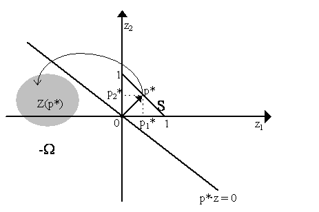
which is the definition of a competitive equilibrium. Q.E.D. § Note, for this proof, that we needed nothing beyond continuity of excess demand functions, Walras's Law and homogeneity of degree zero. We said nothing about the shapes of the excess demand curves, so there can certainly be more than one equilibrium and there is no implication here about it being stable or unstable. It is merely an existence proof. Finally, an interesting result from Hirofumi Uzawa (1962) notes that not only does Brouwer's fixed point theorem imply the existence of a Walrasian equilibrium, but the reverse also holds. Namely, if we define an excess demand function which is continuous, homogeneous of degree zero and where Walras's Law holds and then presume there is a Walrasian equilibrium, that can be translated into a statement of Brouwer's fixed point theorem, i.e. that any function from a non-empty, convex compact space into itself has a fixed point. We do need two troubling assumptions - the strict convexity of preferences and technology ((C.6¢) and (P.6¢)). A more general proof which allows for excess demand correspondences (i.e. set-valued functions) can be found in Debreu (1959: Ch. 5), but for that Kakutani's fixed-point theorem is needed. We turn to it below. (4) Existence of Equilibrium (Kakutani's FPT) We want to be more general and drop the "strict" convexity of preferences and technology but merely "convex" - thus, demands and supplies are "convex sets" rather than particular points. In this case, we end up not with continuous demand and supply functions, but rather with upper-semicontinuous demand and supply correspondences. However, we have placed enough assumptions on production and consumer decisions in our previous sections to guarantee that these correspondences are also convex-valued. As the sum of convex sets is convex and that the sum of upper semicontinuous correspondences are upper semicontinuous, then we know that now the aggregates: x(p) = åh xh(p) y(p) = åf yf(p) e = åh eh are themselves upper-semicontinuous and convex-valued. Thus, we know that: z(p) = x(p) - y(p) - e the aggregate excess demand correspondences are upper semicontinuous and convex-valued. Let us now state the famous "Gale-Nikaido Lemma", due to David Gale (1955) and Hukukane Nikaido Lemma: (Gale-Nikaido) Let p Î S where S is the unit simplex. Let Z(p) represent an upper semicontinuous, convex-valued correspondence from S to Rn and where for all p Î S and z Î Z(p), pz £ 0. Then, there exists a p* Î S such that Z(p*) Ç (- W ) is not empty . Proof: Gale (1955) & Nikaido (1956). (see Debreu, 1959: Th.5.6.1, p.82-3). We go through this proof quite slowly as it is often misunderstood. The condition of the lemma states that the price vector p generates a convex set of excess demands, Z(p), below the Walras' Law constraint pz £ 0. What the Gale-Nikaido lemma claims is that a p* exists such that the generated set Z(p*) intersects the negative orthant, -W . This can be illustrated by the following diagram in a two-dimensional economy:
We are almost there. We have a mapping from the set of prices to the set of excess demands, Z(p). To get to the fixed-point theorem, we must form a mapping back from the set of excess demands to the set of prices. Thus, we need to define one more correspondence. Let us define the following: m(z) = max pz s.t. p Î S M(z) = argmax pz s.t. p Î S This may seem a bit strange, but it is merely an algorithmic mapping. What we do is take a an element z of the set Z(p) and then find the price that "maximizes" its inner product, pz. Recall that prices are restricted to the simplex space S = [0, 1]. Suppose we have two goods only, then a point z in R2 space is z = [zz, z2]. If z1 < 0 and z2 > 0 what set of prices will maximize pz? This is easy: set p1 = 1 and set p2 = 0, and there we have it. Thus, the argmax of the function, M(z) = [1, 0]. What if we are in an n-dimensional commodity space? Then , the algorithm asks that we set the price for every negative zi to zero, and set the price for the positive zis to some positive number (remember the simplex: prices must add up to 1). So, for instance, in n = 3, if z1 < 0, z2 > 0 and z3 > 0, we could have the M(z) = [0, 0.5, 0.5], i.e. we set the price of good 1 to 0, good 2 to 0.5 and good 3 to 0.5. It may look odd, but it is akin to the algorithmic iteration we had in our previous proof. Now, as pz is continuous and S is both upper semicontinuous and lower semi-continuous, then by Berge's Theorem, m(z) is continuous and M(z) is upper semicontinuous. We also know that S is convex. If z = 0, the M(z) = S (convex) and if z is non-zero, then M(z) is some convex portion of S. Thus, M(z) is a convex-valued upper semi-continuous correspondence. Now, let us define the following correspondence: j : (S ´ Rn) ® (S ´ Rn) so, the correspondence j take a price-excess demand pair (p ´ z) and maps it into another price-excess demand pair (p ´ z). The space S is non-empty, convex and compact, the space Rn is non-empty, convex and compact, thus the Cartesian product of the spaces, (S ´ Rn) is also non-empty, convex and compact. Let us now define j (p, z) as: j (p, z) = M(z) ´ Z(p) where, as we have noted earlier, M(z) is convex-valued and upper semicontinuous and Z(p) is also convex-valued and upper semicontinuous. Thus, the Cartesian product of the correspondences, j (p, z) is also a convex-valued, upper semicontinuous correspondence. Thus, we have an convex-valued upper-semicontinuous correspondence from a non-empty convex compact space into itself. By Kakutani's fixed point theorem, there exists a pair (z*, p*) such that (p*, z*) Î j (p*, z*) or, in other words, p* Î M(z*) and z* Î Z(p*). Now, we only need to prove that this fixed point implies the existence of an equilibrium. Thus, once again, we can state this in the form of a theorem. : (Existence) Given a private ownership economy E = {³ h, eh, Ch, qhf, Yf}hÎ H, fÎ F, where all components are defined as before (notably each ³h fulfills axioms (C.1)-(C.6) and each Yf fulfills axioms (P.1)-(P.6)), then there is at least one state of the economy ({xh*}hÎ H, {yf*}fÎ F) and a set of prices, p* Î S such that these form a Walrasian competitive equilibrium, that is zi*(p*) £ 0 for all i = 1, .., n, and xh* and yh* solve their respective optimization problems. Proof: As z(p) = x(p) - y(p) - e are convex-valued upper semi-continuous correspondences, we form the two algorithmic mappings, Z: S ® Rn and M: Rn ® S which are convex-valued upper-semicontinuous correspondences as defined earlier. Form j (p, z) = M(z) ´ Z(p) which itself is a convex-valued upper-semicontinuous correspondence j : (S ´ Rn) ® (S ´ Rn). As (S ´ Rn) is a non-empty, compact convex, set and j is a convex-valued upper semicontinuous correspondence, then by Kakutani's fixed point theorem, there is a (p*, z*) Î j (p*, z*). We now need to show that (p*, z*) forms a Walrasian competitive equilibrium. As z* Î Z(p*), then all elements z of Z(p*) are such that p*z £ 0 (Walras's Law) , thus p*z* £ 0. (by Gale-Nikaido lemma). As p* Î M(z*), then this implies pz* £ p*z* for all p Î S by the definition of M(z*) as the argmax. Thus, by Walras's Law, this implies pz* £ 0 for all p Î S. This last part is important: for all p this will be true. Suppose, then, we take the following price vector p = [1, 0, 0, ....0] Î S (a price vector with 1 in the first place and zeroes everywhere else). This implies that pz* = z1* £ 0 - equilibrium in the first market! Let us proceed and take another price vector p = [0, 1, 0, ....0] Î S (a price vector with 1 in the second place and zeroes everywhere else). This implies that pz* = z2* £ 0 - equilibrium in the second market! Proceed by these steps, and we can see that this implies that z* £ 0, i.e. equilibrium in all markets. Thus, our fixed point p*, z* is an equilibrium.§ There is one important thing to note: z* £ 0 implies that Z(p*) intersects the negative orthant (Gale-Nikaido), but recall that this is a correspondence. This means that z* is only one of the various excess demand vectors that the price p* is going to yield. It does not say that at p* people will choose the particular market clearing demands z* to effectuate their trades, thus, even at the equilibrium price, we may have a market disequilibrium. In sum, all Arrow-Debreu tells us is simply that it is possible (but not necessarily likely) to trade at equilibrium (markets clear) when price is p*, but it does not mean more than that. For a constructive proof, which provides the numerical solution of the equilibrium, we refer to the work of Herbert Scarf (1973). Other References Kenneth J. Arrow and Frank H. Hahn (1971) General Competitive Analysis. Amsterdam: North Holland. Gerard Debreu (1959) Theory of Value: An axiomatic analysis of economic equilibrium. New York: Wiley. Gerard Debreu (1982) "Existence of Competitive Equilibrium", in Arrow and Intriligator, editors, Handbook of Mathematical Economics, Volume II. Amsterdam: North-Holland. David Gale (1955) "The Law of Supply and Demand", Mathematica Scandinavica, Vol. 3, p.155-69. Tjalling C. Koopmans (1957) Three Essays on the State of Economic Science. New York: McGraw-Hill. Harold W. Kuhn (1956) "On a Theorem by Wald", in H.W. Kuhn and A.W. Tucker, editors, Linear Inequalities and Related Systems. Princeton: Princeton University Press. Hukukane Nikaido (1956) "On the Classical Multilateral Exchange Problem", Metroeconomica, Vol. 8, p.133-45. Hukukane Nikaido (1968) Convex Structures and Economic Theory. New York: Academic Press. Hirofumi Uzawa (1962) "Walras's Existence Theorem and Brouwer's Fixed Point Theorem", Economic Studies Quarterly, Vol. 12 (2), p.59-62.
|

All rights reserved, Gonçalo L. Fonseca