The Harrod-Domar Model

________________________________________________________

"If the aggregated result of trial and error by numerous producers gives a value of G [actual growth] which is different form G_w [warranted growth], there will not be any tendency to adapt production towards G_w, but, on the contrary, a tendency to adapt production still further away from it whether on the higher or lower side."

(Roy F. Harrod, Towards a Dynamic Economics, 1948: p.87)

"Faced with this difficulty [instability], I have been tempted...to enquire whether it is not possible, by some modification of Mr. Harrod's assumptions, to overcome the deficiency. The prize is a great one, for no one can study Mr. Harrod's work at all deeply without feeling that results of really great significance are just round the corner."

(John Hicks, "Harrod's Dynamic Theory", 1949, Economica)

"I hope that we shall hear no more of the "Harrod knife-edge." ...[T]his instability principle...is only one part, and perhaps by now a minor part, of my total growth theory."

(Roy F. Harrod, "Reply to Robinson", 1970, Economic Journal)

Back

Contents

(1) Keynes and Oxbridge
(2)

(1) Introduction
(2) The Solow-Swan Growth Model
(3) Adding Depreciation
(4) Solving the System
        (A) The Cobb-Douglas Solution
        (B) The General Solution
(5) Adjustment Processes: Solow vs. Harrod 

The heroic entrepreneurs of Schumpeter are resurrected, only slightly less heroically, in the General Theory (1936) of John Maynard Keynes. Investment, in the Keynesian system, is an independent affair contingent upon financial conditions and the "animal spirits" of entrepreneurs.

Keynes did not extend his macroeconomic theory into the longer run. By this we mean that Keynesian macroeconomic equilibrium was contingent upon a given stock of capital. But as there is positive investment in Keynes's equilibrium, then there must be changing capital stocks. Thus, the macroeconomic equilibrium of today will be different from the macroeconomic equilibrium of tomorrow. Keynesian macroeconomic equilibrium could not, in this sense, be "permanent"; it is merely "short-run".

Sir Roy F. Harrod was perhaps the first to notice this and it was Harrod (1936, 1939, 1948) who initiated the move from short-run macroeconomic equilibrium to longer-run theories of growth and cycles. We have referred to this elsewhere as the "Oxbridge" research program" research program, in recognition of the fact that this program was initiated by Oxford economists Roy Harrod and John Hicks, and continued by Cambridge economists such as Joan Robinson, Nicholas Kaldor and Luigi Pasinetti.

Although developing a Keynesian theory of business cycles was arguably the primary objective of the Oxbridge researchers, it is perhaps their contributions to growth theory that have had the wider impact. It is interesting to note that the Oxbridge program was the first such attempt in the English-speaking world since John Stuart Mill a full century earlier!

The two contributions that kicked off the growth side of the program were the models of Roy Harrod (1939) and Evsey Domar (1946). Although their final solution happens to be the same, the Harrod and Domar models are actually constructed differently, and thus we consider them separately. We turn to the Cantabrigian (Kaldor, Robinson, Pasinetti, etc.) contributions later. For those wishing to skip the intermediate steps, we draw your attention to Section (5) which contains the "modern" (but inaccurate) version of the Harrod-Domar growth model.

(A) Macroeconomic Instability

We consider first Roy Harrod's (1939, 1948) construction. There have been numerous formalizations of Harrod's model. In this section, we will just present a heuristic version of his theory, postponing the various formalizations of Harrod's theory until later.

Harrod's main objective was to integrate the Keynesian theory of the multiplier with the investment accelerator [for an excellent account of Harrod's vision of economic dynamics, see Besomi (1999)]. The Keynesian multiplier tells us that investment generates aggregate demand and consequently output and savings. But the investment accelerator -- what Harrod called "the Relation" -- tells us that investment is driven by expected changes in aggregate demand. Harrod's basic question was the following: what happens when these expectations are not fulfilled?

Why this is a problem should be apparent. On the basis of the accelerator, entrepreneurs invest in the expectation that future demand will be some particular amount. If they invest too much, they will experience accumulating inventories and take this as a signal to reduce investment. But, by the Keynesian multiplier, that very decrease in investment will reduce aggregate demand and output further, thereby leading (by the accelerator) to further reductions in investment in the future and so on. In contrast, if the entrepreneurs' initial expectations are too low, then they will invest too little and consequently observe their inventories depleting quickly and thus boost their investment. But, once again, by the multiplier, that very increase in investment will lead to a further rise in aggregate demand, and thus, by the accelerator, greater investment and further aggregate demand growth, and so on.

In sum, we see, then, that the interaction between the multiplier and the accelerator can lead to upwards or downwards instability depending on the initial configuration of entrepreneur expectations. If initial expectations are "too high", then there will be an spiraling decline in investment and output. If initial expectations are too low, we get an explosive expansion. If, however, these expectations are "just right", so that aggregate demand growth is expected by entrepreneurs to be exactly what turns out to be the case, then we have a case of "balanced" or "steady-state" growth.

Roy Harrod (1939, 1948) presented this idea in a rather simple model. He defined

where s is the propensity to save out of income. Notice that this is nothing other than the simplest Keynesian multiplier.

Now, Harrod differentiated between actual (ex post) investment, I_a, and planned (ex ante) investment, I. These two magnitudes need not be the same. Actual investment is planned investment plus any unplanned accumulation/depletion of inventory stocks,

I_a = I + DV

where DV are the changes in inventory. Harrod then introduces the following ratio:

v_a = I_a/DY

where we can think of v_a as the actual "marginal" capital-output ratio, "the increment of capital per unit increment of output actually produced" (Harrod, 1939: p.258). Notice that v_a is an ex post term. As a result, actual growth, denoted g, can be written as:

g = DY/Y = s/v_a

Notice that this equation is a mere truism since it arises from the national accounting identity I_a º S.

Harrod then introduced the ratio v to indicate the value of v_a where there is no undesired accumulation/depletion of inventories. In other words, if v_a = v, then expectations of entrepreneurs are fulfilled. He defined the warranted rate of growth, g_w as:

g_w = s/v

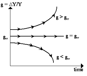
so the warranted rate is "the over-all advance which, if executed, will leave entrepreneurs in a state of mind in which they are prepared to carry on a similar advance," (Harrod, 1948: p.82).

The dynamics of the accelerator story follow verbally. If g = g_w, then we are saying that actual investment is equal to planned investment and so expectations are fulfilled and entrepreneurs have no incentive to adjust them. If, in contrast, g > g_w, actual output growth exceeds the warranted rate. Going through the equations, this means that s/v_a > s/v Þ I_a< I, i.e. actual investment (I_a) is less than planned investment (I). In other words, too much output growth (think of this as too much aggregate demand growth) means that entrepreneurs will find their inventories depleting and their production lines stretched and so they will feel that they have not invested enough. But by investing, we know from the multiplier relationship that this will increase output further and thus push g further above g_w. In contrast, if g < g_w, then I_a > I. In other words, too little output growth means that actual investment exceeds planned investment, i.e. inventories are accumulating and production equipment is lying idle. Entrepreneurs, thinking that they have invested too much, will cut down on their future investment plans. By the multiplier, this will push g further below g_w.

Thus, Harrod's story has a built-in instability arising from the macroeconomic relationships of the multiplier and accelerator. This is depicted in Figure 1. If the economy begins at actual growth rate g = g_w, then we stay on the balanced growth path forever. But if the initial actual growth rate is different from the warranted, g ¹ g_w, then the economy will move inexorably in either an upward or downwards direction forever. This macroeconomic instability property has become known as "Harrod's knife-edge".

Fig. 1 - Harrod's Knife-Edge

(A) Jorgensen's model

Harrod's (1939, 1948) story of macroeconomic instability was told in a rather simple and verbal manner. Instability is a property of some underlying dynamical system that was not made explicit. As such, it might be worthwhile examining Harrod's model and conclusions a bit more formally. As it happens, the famous Harrod instability result depends on the formalization we use. We shall pit two versions against each other -- one by Dale W. Jorgensen (1960) which confirms instability under certain conditions, and another by Hugh Rose (1959) which disputes this conclusion.

Jorgensen's (1960) formalization of the Harrod model begins with the assumption that planned savings are a function of lagged income:

S_t = sY_t-1

This is the multiplier relationship. The accelerator is captured by the following equation relating planned investment to actual changes in income:

I_t = v(Y_t - Y_t-1)

where s is the marginal propensity to save and v is the accelerator coefficient.

This system, encompasses the "expectations" idea we gave earlier. To see this, note that when expectations are fulfilled, the macroeconomic equilibrium is satisfied, implying that planned savings is equal to planned investment, I_t = S_t, so:

sY_t-1 = v(Y_t - Y_t-1)

thereby yielding the simple first order linear difference equation:

Y_t - [1 + s/v]Y_t-1 = 0

The solution to this is merely:

Y_t = A[1 + s/v]^t

where A is a constant derived from the initial value of Y_t. This states that output grows at the steady rate s/v. Thus, it is from this that we assert that s/v is the warranted rate of growth, i.e. the rate of growth which maintains macroeconomic equilibrium (i.e. leaves expectations fulfilled).

Now, we need to show that instability results when g ¹ g_w. We do this naïvely. Suppose that actual income at t, Y_t^a, is different from the income necessary for warranted growth, i.e. suppose Y_t^a ¹ A[1+s/v]^t. Defining:

D_t = Y_t^a - A[1+s/v]^t

then if D_t > 0, actual income is greater than warranted income (and vice versa if D_t < 0). Suppose that we are growing at the warranted rate and all of a sudden, income increases "accidentally" by D_t. In this case, savings remain S_t = vY_t-1, or:

S_t = sA[1+s/v]^t-1

but investment, I_t = v(Y_t - Y_t-1) must be modified to:

I_t = v(A[1+s/v]^t + D _t - A[1+s/v]^t-1)

Doing some acrobatics with the investment equation, we see that it becomes:

I_t = vA([1+s/v]^t - [1+s/v]^t-1) + vD_t

= vA((1+ s/v)[1+s/v]^t-1 - [1+s/v]^t-1) + vD_t

= vA(s/v)[1+s/v]^t-1 + vD_t

or simply:

I_t = sA[1+s/v]^t-1 + vD_t

which, notice, from the definition of savings, implies that:

I_t = S_t + vD_t

As we proposed D_t > 0, then I_t > S_t, i.e. investment exceeds savings. Consequently, by the Keynesian multiplier, output in the next period will rise, i.e. Y_t+1 > Y_t. However, recall that we initiated this whole thing with an accidental rise in output (D_t > 0). Thus, we have output instability: if output is greater than warranted output, it will generate excess investment and thus, by the multiplier, a further increase in output and so on. Conversely, if D_t < 0, so that output accidentally falls below warranted output, then this will generate excess savings and, by the multiplier, a further decline in income. Thus, our warranted path is unstable in the sense that if we are not on it to begin with, then we deviate further away from it as time proceeds.

We can formalize what has just been said as follows. Let us define the disequilibrium process as D_t+1 - D_t = g D _t where g > 0, so that if D_t > 0 (income is above the path, and so there is excess investment), then output increases and leads to a greater amount of excess investment. Formally we can define a simple difference equation:

(i) D_t = (1+g )D_t-1

Now, excess investment was defined as:

D_t = I_t - S_t

where I_t and S_t are planned magnitudes. Thus, substituting in for I_t, S_t and D _t:

(1+g )D_t-1 = v(Y_t - Y_t-1) - sY_t-1

which, upon rearrangement, yields:

(ii) Y_t = [1 + s/v]Y_t-1 + [(1+g )/v]D _t-1

So, now we have a system of two difference equations, (i) and (ii). We can reduce this to a single system in income. Namely, recognizing that (ii) can be expressed as:

(ii¢ ) [v/(1+g )]Y_t - [(v + s)/(1+g )]Y_t-1 = D_t-1

so, iterating forward by one period:

[v/(1+g )]Y_t+1 - [(v + s)/(1+g )]Y_t = D_t

so, using the equality in (i)

[v/(1+g )]Y_t+1 - [(v + s)/(1+g )]Y_t = (1+g )D_t-1

and then plugging in (ii¢ ) again:

[v/(1+g )]Y_t+1 - [(v + s)/(1+g )]Y_t = (1+g ){[v/(1+g )]Y_t - [(v + s)/(1+g )]Y_t-1}

or:

[v/(1+g )]Y_t+1 - [(v + s)/(1+g ) + v]Y_t + (v + s)Y_t-1 = 0

and rearranging again and iterating one period back:

Y_t - [(1+ s/v) + (1+g )]Y_t + [(1 + s/v)(1+g )]Y_t-2 = 0

which is a second-order difference equation in output. The solution to the system is:

Y_t = A(1+s/v)^t + B(1+g )^t

where A and B are constants relating to initial conditions. Now, this system can be stable or unstable depending on the relative values s/v and g . Now, we know s/v > 0 and g > 0, but that is about it. If s/v > g , that means that the first root (1+s/v) eventually dominates, and the output path returns to its equilibrium, steady-state path (with growth at the warranted rate s/v). But if g is big enough so that s/v < g , then (1+g ) eventually dominates and the output path approximates the path (1+g ) > 1, and thus becomes unstable (or rather, moves away from s/v).

Jorgensen's (1960) conclusion, then, is that it is necessary that the rate of excess demand growth (g ) must be greater than the warranted rate of growth (s/v) in order for the Harrodian system to be unstable. He shows that an earlier "proof" of Harrodian instability by Sidney Alexander (1950) hinges on his implicit assumption that g > s/v.

(B) Rose's model

Hugh Rose (1959) provided a different formalization of Harrod's model which proposed a different disequilibrium mechanism and obtained stability. Rose worked on the Hayekian rather than the Keynesian conception of investment: in other words, he presumed investment plans were made as an "adjustment" to an optimal capital stock, K*. The following formalization of Rose's model is derived from Hahn and Matthews (1964).

Let K_t* be the desired capital stock at time t. The desired capital stock is governed by the expected growth of output. Let us suppose that entrepreneurs expect output to grow at the warranted rate s/v, so the desired capital stock grows at the same rate. Then, starting at t, the desired capital stock m periods ahead will be:

K_t+m* = K_t*^(s/v)m

Now, suppose entrepreneurs at t have a shortage of capital and they want to "catch up" with their desired capital stock by time t+m by fixing a rate of investment that will take them there. Let g be the chosen (constant) rate of capital accumulation, i.e. g = (dK/dt)/K. Thus starting at K_t and choosing a particular rate g, the capital stock at t+m will be:

K_t+m = K_t^gm

As they want to catch up to desired capital in m periods, then:

K_t+m = K_t+m*

or:

K_t^gm = K_t*^(s/v)m

taking logs:

ln K_t + gm = ln K_t* + (s/v)m

so:

g - s/v = (1/m)(ln K_t* - ln K_t)

but now recognize that by definition:

g - (s/v) = d(ln K_t - ln K_t*)/dt

so the equation can be rewritten as:

dk /dt = -k /m

where k = ln K_t - ln K_t* = ln (K/K*). The solution to the simple first order linear differential equation in k is:

k (t) = k ₀e^-t/m

where k ₀ is the initial k . Notice that as -1/m < 0, then this system is stable, i.e. k (t) ® 0 as t ® ¥ , or translated, as ln(K/K*) ® 0, implies K/K* ® 1, or simply K(t) ® K(t)*, so that the actual capital stock approaches the desired capital stock. Letting output be translated simply as a Y(t) = ¦ (K(t)), then we obtain stability of the output growth path.

This stability result is striking. What is going on? Well, it rests on the assumption that all desired investment is met and that expectations are consistent with warranted growth path. This is not consistent with the original Harrod model or its Jorgensen formalization. A.W. Phillips (1961, 1962) restored Jorgensen's distinction between actual and desired investment into Rose's model and obtained instability (although, once again, noted that instability depended on the condition that g > s/v).

In sum, it seems that Harrod's theory yields instability. But it rests crucially on the assumption that the instability-causing excess demand process, captured by parameter g , exceeds any tendency to return to the warranted growth path.

Back

Top

Selected References

Next