|
________________________________________________________
________________________________________________________ As outlined in our introduction, Arthur C. Pigou's (1920) assertion that myopic agents might "save too little" was taken up by the brilliant young Cambridge philosopher, Frank P. P. Ramsey (1928) -- long before growth theory came into its own. Ramsey's main concern was to determine the optimal rate of savings and then show how myopic agents would not achieve that optimum. But what is the optimal rate of savings? Ramsey's exercise was explicitly grounded in Benthamite utilitarianism. He sought to find the allocation across generations which maximized social welfare -- with "social welfare" defined as the sum of utilities of people in a society. From the social welfare-maximizing allocation, we will be able to determine an "optimal" rate (or rather, path) of saving. However, this comes up against traditional Benthamite problem of defining exactly whom constitutes "society". This is particularly pertinent in a growth context as the issue of balancing the interests of current and the future members of society is a critical ingredient. It is obvious that we can maximize the social welfare of the current generation by having them simply consume all their income, but then there would be no savings and thus no capital to generate income for the next generation. Like Arthur Pigou (1920), Frank Ramsey argued that "society" is composed of everybody in every generation, current and future, and that they all should be given equal weight in the social welfare function. Now, as we outline later, a direct Benthamite sum of utilities yields the problem that this sum can be infinite -- and infinities cannot be compared, and thus an optimum might not be found. Adding a time discount factor would solve the problem, but Frank Ramsey considered time discounting as "a practice which is ethically indefensible and arises merely from the weakness of the imagination" (Ramsey, 1928). Time preference, as Pigou (1920: Pt I, Ch. 2) originally asserted, is a personal weakness which should not be imported into a normative exercise. (see our review of "intertemporal social welfare" for more details). However, Ramsey recognized that by omitting time preference, the problem of non-comparability of infinite sums emerged. In its stead, he introduced the ingenious device of "bliss points". Specifically, he defined a social unwelfare function of the following sort:
or, in continuous time:
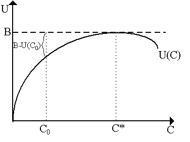
where B is the "bliss" level of utility, assumed to be the maximum utility achievable for a generation. This is the same across generations. Note that [B - U(Ct)] is the distance away from bliss that generation t is if it consumes Ct: the smaller [B - U(Ct)] is, the "better off" the generation is. We can see the utility function in Figure 1. When C = C*, then we are at "bliss" in the sense that marginal utility is zero, U¢ (C*) = 0, so that increasing consumption beyond this reduces utility (or, more generally, does not increase it). At lower consumption levels, such as C0 in Figure 1, B > U(C0), and U¢ (C0) > 0.
Consequently, for a social optimum, we wish to find the consumption allocation across generations for which R is minimized. This, Ramsey asserted, side-steps the issue of "infinite sums", but, as we shall later, it is actually doubtful that the Ramsey device is foolproof. Let us proceed with the Ramsey exercise. Thus far, we have only some idea of what the Ramsey social welfare function is. Now, we need to add the rest of the economy. In macroeconomic equilibrium, aggregate demand is equal to aggregate supply, or Y = C + I. As I = dK/dt and Y = F(K, L), then:
forms the "real economy" constraint which our society faces. Thus, consumption paths must be feasible in this manner. Now, Ramsey (1928) included the disutility of labor supply into his utility function, so letting U(C) be the utility of consumption and V(L) the disutility of labor supply, Ramsey combined them in an additively separable manner, i.e. u(C, L) = U(C) - V(L), where U¢ > 0, U¢ ¢ < 0 and V¢ > 0 and V¢¢ > 0. Consequently, defining B as "bliss", we mean that [U(Ct) - V(L)] £ B for all acceptable Ct and thus, note, U¢ (C) = 0 when U(C) - V(L) = B (i.e. at bliss, marginal utility of further consumption is zero). The distance from bliss for any generation t is [B - U(C(t)) + V(L(t))]. Ramsey then set out his social welfare problem in minimization form as:
where K0 is the initial capital stock. The problem can be thought of as following. Social welfare is maximized if every generation is "at bliss". However the society's initial capital stock K0 (and thus the initial income) may be too low to achieve bliss levels of consumption immediately. Consequently, we might be interested in achieving bliss as quickly as possible by holding back consumption and producing a lot of capital today. The more we save now, the sooner society will reach bliss. But this is a bit unfair for the first few generations who must sacrifice their own consumption to ensure quicker convergence to bliss. Consequently, the "cost" of achieving bliss quicker is the consumption utility that the initial generations lose in their sacrifice. Balancing quick convergence to bliss with the utility cost of foregone consumption is the heart of the Ramsey problem. The solution follows standard calculus of variations techniques -- a mathematical tool which, incidentally, Ramsey (1928) was among the first to introduce into economics. For simplicity of notation, let K¢ = dK/dt and L¢ = dL/dt and let the intergrand be denoted:
So, substituting in our constraint:
Defining IL = dI/dL and IL¢ = dI/dL¢ and equivalently for IK and IK¢ , then:
Euler equations are the solution for calculus of variations problems. For our particular problem, we have the following pair of Euler equations:
which hold for all t ³ 0. The first Euler equation reduces simply to:
so that, at every t, the marginal disutility of labor must be equal to the marginal product of labor multiplied by the marginal utility of consumption. The second equation reduces to:
so that at every t, the marginal product of capital is equal to the negative of the growth rate of marginal utility of consumption. Now, since I is time-autonomous, then we apply the well-known result that:
where a is some constant. Thus:
But what is a ? For this we need the transversality conditions. There are two of them. The first is merely:
which, substituting in, yields:
so (net) utility approaches bliss in the limit, i.e. [U(C) - V(L)] ® B as t ® ¥ . The second transversality condition is that:
But from before, we know that I - K¢ IK¢ = a , so by substitution:
But as a is a constant, independent of time, then it must be that a = 0 for all t. Thus, returning back to our equation we see:
so, solving for K¢ :
This is the famous Keynes-Ramsey Rule for dynamic efficiency. Specifically, this states that the optimal amount of investment at any time t (K¢ ) is equal to the distance-from-bliss divided by the marginal utility of consumption. If we ignore labor L (or rather assume labor is supplied inelastically), then this reduces to:
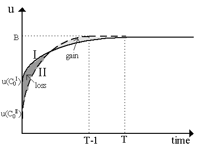
What does this mean? Intuitively, suppose that we decide to "speed up" society's convergence to bliss. In other words, let us force the current generation to save amount K¢ so that one extra generation will be at bliss in the future. The net gain of that future generation is B (its new, blissful utility) minus U(C) (the utility it would have otherwise), i.e. B - U(C). As this is positive, it might always seem worthwhile to do to so. But the cost of "speeding up", as we stipulated, was the consumption foregone by the initial generation. If they save amount K¢ , then U¢ ·K¢ is the cost of speeding up convergence by one generation. Optimally, then, the marginal (net) benefit of speeding up, B - U(C), must be equal to the marginal cost of doing so, U¢ ·K¢ . That is the Keynes-Ramsey rule. This can be illustrated heuristically by appealing to Figure 2. We have depicted two utility paths I and II, both of which achieve bliss B after some time. Path I (solid line) converges to bliss at time T, but Path II (dashed line) converges to bliss one period earlier, at T-1. But notice that Path I also starts at a higher consumption and thus utility than Path II, U(C0I) > U(C0II). Path II converges to bliss faster than Path I, but it sacrifices the utility of the early generations. Thus, the "gain" of using Path II is the speeded-up convergence to utility and thus the utility gains of the generations around T-1 (captured by the lightly shaded area in Figure 2), while the "loss" of using Path II is the foregone higher utility of the earlier generations (captured by the darkly-shaded area in Figure 2). The Keynes-Ramsey rule asserts merely that the optimal path will be that where the marginal gain of speeding up is equal to the marginal cost of doing so. [Note: the prefix "Keynes" is added to this result because of Ramsey's gracious acknowledgment to John Maynard Keynes for coming up with the interpretation we just provided].
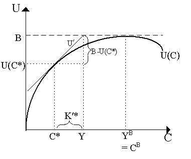
[Note: We could have solved the Ramsey problem via optimal control methods, setting up a Hamiltonian H = [B - U(C) + V(L)] + l [F(K, L) - C] where l is the costate variable, and so on. Karl Shell (1969) makes the curious assertion that this Ramsey problem does not fulfill the traditional transversality condition of infinite-horizon problems, limt® ¥ l (t) = 0. This is not quite right, however.] There are a few interesting features worth noting. Firstly, note that the Keynes-Ramsey rule is independent of the pricing of factors, specifically it is independent of marginal product of capital (as Ramsey (1928) was quick to emphasize). Intuitively, all we need to know for the rule is the initial capital stock, K0, the shape of the utility function, U(C), and the bliss level, B, and we can derive the optimal consumption path. To see this, examine Figure 3, where we have redrawn our utility function. As K¢ = Y - C, then the Keynes-Ramsey rule becomes
So, for a given Y, we can deduce the optimal consumption C* by finding the level of consumption for which this is true. This is shown in Figure 3.
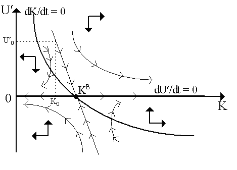
Notice, from Figure 3, that at the bliss point, all output is consumed (YB = CB). This will be approached asymptotically. Specifically, suppose that in Figure 3, Y is the initial level of income (i.e. Y = F(K0), where K0 is the initial capital stock). As Y = F(K0) > C*, then K¢ * > 0, so capital increases and thus pushing output further to the right along the axis (and consumption along with it). Thus, over time, Y ® YB and C ® CB asymptotically (as K¢ ® 0, it declines in size during the process). Notice that the "bliss" point corresponds to what was later called Golden Rule growth. But note that now we obtain Golden Rule growth not by choosing among the Solowian steady-states, but starting from any arbitrary initial position. Thus, by endogenizing the propensity to save via the Benthamite social welfare function, the Golden Rule equilibrium becomes stable. We can represent the dynamics of the Ramsey model via the phase diagram in Figure 4. Omitting labor, we can rewrite our Euler equation for capital as:
which is a differential equation in U¢ . Recovering our constraint, we obtain a second differential equation:
For simplicity, let us assume that C = C(U¢ ), so consumption is a function of marginal utility (so U must be smoothly invertible, as it is in Figure 3 above). Thus we have a system of two differential equations in U¢ and K. Consider dU¢ /dt = -FK·U¢ first. In steady state, dU¢ /dt = 0, so -FK·U¢ = 0, which implies that either FK = 0 or U¢ = 0. We assume that FK > 0 for all K (diminishing marginal productivity everywhere), then it must be that U¢ = 0 (and, if U¢ = 0, recall, we are at "bliss"). In (K, U¢ )-space in Figure 4, then, the isokine for dU¢ /dt = 0 will be the horizontal axis (where U¢ = 0 and K is indeterminate). The disequilibrium dynamics are easy to decipher. Note that:
so above the dU¢ /dt = 0 isokine, U¢ has a tendency to fall, whereas below the isokine, U¢ will rise. Thus, the vertical directional arrows in Figure 4.
Now, consider the second differential equation. In steady-state, dK/dt = 0, which implies that F(K) = C. As C = C(U¢ ) which is invertible by construction, then the isokine dK/dt = 0 will have a form U¢ = C-1(F(K)) and slope dU¢ /dC < 0 (diminishing marginal utility of consumption). This is shown by the downward-sloping dK/dt = 0 isokine in Figure 4. The disequilibrium dynamics for the dK/dt = 0 isokine can be deciphered by noting that:
so that to the right of the dK/dt = 0 isokine, K rises, while to the left of it, K falls. Thus the horizontal directional arrows in Figure 4. Together, the isokines dK/dt = 0 and dU¢ /dt = 0 have underlying dynamics which resemble a "saddlepoint": there is a single stable arm going to the steady-state equilibrium (0, KB), but all other paths move away from it. Notice that the steady-state (U¢ , K) = (0, KB) is "bliss" as U¢ = 0, so KB is the level of capital corresponding to bliss. Saddlepoint dynamics imply that, beginning at some initial capital level K0, we can define a unique level of marginal utility, U¢ 0 which puts us on the stable arm (and this chosen U¢ 0 corresponds to choosing an optimal initial consumption, C0, as we had earlier in Figure 3). As time progresses, and we continue choosing consumption rates and thus utilities so that we stay on the stable arm, we move towards the steady-state (0, KB), so that K ® KB and U¢ ® 0, i.e. we are approaching bliss asymptotically. The Ramsey (1928) exercise remained dormant for the next half-century. It was resurrected in the 1950s and 1960s, when the emergence of growth theory resurrected some of the questions Ramsey had asked. The first result, the simplest result, was the determination of the "Golden Rule" of growth.
|
All rights reserved, Gonçalo L. Fonseca


