|
Contents (A) Compound Interest In two separate books, Knut Wicksell (1893, 1901) tried to present Böhm-Bawerk's theory carefully and found a considerable objection. Specifically, as Wicksell notes in his Lectures on Political Economy (1901: p.184), the average period of production is not independent of the rate of interest if we use compounding to calculate the average time distance between input and output. To see this, let us take an example from Lutz and Lutz (1951): let there be a process which lasts two periods and that in the first period I units are applied (and congealed for two periods) and in the second period I units are applied (and congealed for a period). Now, recall that Böhm-Bawerk's formula for the average period of production was:
which in our case reduces to:
Now, let us propose that for every period an input is congealed in the process, it yields a rate of interest, i. If we use a simple interest formula, then:
which, solving for q , yields q = 1.5. Thus, Böhm-Bawerk's formula for the average period of production is compatible with simple interest. However, as Wicksell (1901: p.184) notes, with compound interest things change. Specifically, with compound interest, then:
which, solving for q , yields:
which is very different from Böhm-Bawerk's formula. The actual solution here is 1.51 if we take i = 10% -- close but different, and will be even more different with a more complicated production processes. We see immediately that with compounding, the average period of production q is dependent on the rate of interest, i, whereas for Böhm-Bawerk's case, it was not. Thus the interest rate, an outcome of Böhm-Bawerk's system, actually comes in also as a determinant. In various ways, this problem is conceptually akin to that unearthed by "Price Wicksell effects" in the Cambridge Controversy. (B) The Optimal Production Period Consequently, Wicksell (1901: p.172-84) abandoned Böhm-Bawerk's method and reverted to an "absolute" period of production - or what can be referred to as "point input-point output" where all inputs are implemented together at one time, and all output emerges together at another time. Consequently, the determination of the "optimal period of production" means something different for Wicksell. His famous examples of "wine" or "timber" aging can be used to illustrate this. Wine or timber grows in "output" (qualitatively for a barrel of wine and quantitatively for a tree) over time. To take a simplistic case, let I be "input" at the initial time period (t = 0) and let us denote output by Y = I¦ (t) where ¦ (t) is some continuous function of time. As we shall see, ¦(t) can have quite a variety of admissible shapes. As we have a homogeneous commodity, then we can normalize sale price to 1 and so Y = I¦(t) also represents the growth in the sale value of output. Thus, present value of the output, then is:
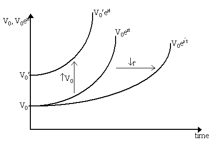
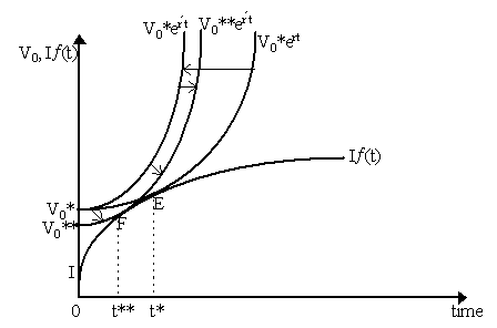
Obviously, as I¦(t) rises and/or r falls, then V0 increases. Diagramatically, we can conceive of present value as in Figure 1. Let X be some amount of earnings per period that grow at an exponential rate r over time. Then the present value of a stream Xert is merely V0 = (Xert)e-rt = X. Thus, for a given r and earnings per period X (= V0) we can draw out a curve V0ert which can be conceived as an "isovalue" curve, i.e. a series of combinations of V0ert and t which yield the same present value V0. As time increases, total earnings increase so that V0ert increases. Thus, the isovalue curve is upward sloping and convex.
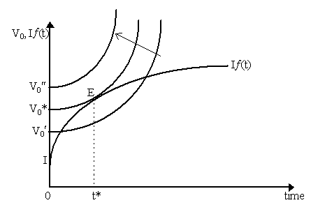
We can easily see what increasing returns per period (increasing our old X, now V0) or increasing r will do. If, for some reason, earnings per period increase from V0 to V0¢ , then discounted backwards at the same interest r, present value increases from V0 to V0¢ - this is an upward shift in the isovalue curve as we see in Figure 1. If, on the other hand, earnings per period V0 stay the same but r falls, then the discounted value and thus the intercept will still be the same, but the curve will swing outwards because as we obtain the same amount of earning per period, it now takes a longer amount of time (and thus more total earnings) to acquire the same present value of them. The main thing to note, for our purposes, is that a given rate of interest r defines an "isovalue map" of curves V0, V0¢ , V0¢ ¢ etc. of the same shape but of different intercepts. Thus, as we move to the northwest, the present value (V0) increases (as is shown heuristically in Figure 1). Consequently, when we specify the function I¦(t) (with intercept I where I can be thought as the "acorn", and I¦ (t) the size of the tree that grows over time - as in Figure 2 below), then we are faced with a very simple optimization problem, namely:
namely, we attempt to find the optimal t* (the date at which we chop the tree, or bring the wine to market) that maximizes the present value of the earnings stream. Diagramatically, this is equivalent to finding the highest isovalue curve (for a given r) that is feasible for a given I¦ (t). This is shown heuristically in Figure 2 at point E, where V0* is optimal isovalue curve and thus the maximum present value that can be achieved.
Now, in this diagram we have assumed a concave shape for the I¦ (t) curve. This is not necessarily always the case. To see the result of the optimization problem more clearly, let us normalize the "acorn" out, so let I = 1 so that we now face:
then the first order condition for a maximum is merely:
or simply:
Now, recall that ¦¢ = d¦ (t)/dt, thus ¦¢ /¦ is merely the growth rate of output - i.e. "g". Thus the condition first order condition yields the infamous "Golden Rule" of growth theory (what Wicksell (1901: p. 178) called "Jevons's well-known formula"), that the rate of interest be equal to the rate of growth. It is easy to realize that this condition is the tangency condition implied in Figure 2 between the V0* isovalue curve and I¦ (t). Now, the second order condition for a maximum implies that:
or simply that:
thus, we see immediately that ¦¢¢ need not be negative but merely small - thus the concavity of ¦ (t) function, as we drew it in Figure 2, is not really implied. It might be worthwhile doing some comparative statics - in particular, finding out what the impact of increasing the interest rate, r, implies. As we see, totally differentiating the first order condition, we obtain:
where, note, the numerator is positive but what about the denominator? Well, by combining second order condition and the first order condition, we can see that ¦¢¢ /¦¢ < r = ¦¢ /¦ , thus cross multiplying, ¦¢¢¦ < ¦¢ 2, thus the denominator is negative, so dt/dr < 0, i.e. a rise in the rate of interest will lead to a shortening of the optimal production period. There is one final implication of Wicksell's schema. The way we have set it out, we were attempting to maximize present value subject to the I¦ (t) constraint with r constant. Alternatively, we could have tried to maximize the rate of profit r subject to ¦ (t) given V0 constant. We would have achieved, under most circumstances, the same result, t*. Thus, maximizing present value or maximizing the "internal rate of return" (which is what is implied by the second exercise) will yield the same result. To see this, recall that V0 = ¦ (t)e-rt can be expressed for r as an optimization problem so:
for which the first order condition implies:
or simply, ¦ ¢ /¦ = r, which is the Golden Rule once again. Wicksell (1901: p.172ff) himself used this method to solve his system rather than maximizing present value - as indeed did virtually all contemporaries such as Böhm-Bawerk, Knight and Hayek. Maximizing present value, the more common approach today, stems largely from Fisher, Keynes, and Hicks. (C) Real and Price Wicksell Effects There is an additional concern that must be raised here -- namely, the issue of "Wicksell Effects" made so familiar in the Cambridge Capital Controversy of the 1960s. Recall that in the Cambridge controversy, the term "Real Wicksell Effect" was used to denote a situation when a change in the rate of profit results in changes in capital intensity in real terms while a "Price Wicksell Effect" is when a change in the rate of profit leads to a change in capital intensity in value terms. A rise in the rate of profits, in our context, reduces the optimal period of production, t, but it also reduces what we shall distinguish as the "physical" (K) and "value" (pK) volumes of capital for a given amount of labor (assumed constant throughout). But did not the Cambridge controversy have something to do with heterogeneous capital? We can understand this more clearly if, following Ahmad's (1991) suggestion, instead of conceiving of I¦ (t) as the time path of a single tree, we consider it the profile of a "forest" with many trees of all different ages. Thus, at any particular ti, we have I¦ (ti) amount of trees of that particular age (or rather, not "number" of trees, but "amount of timber ingrained in trees of that vintage"). Thus, t* does not denote the "cutting time" for a single tree, but rather it represents the optimal composition of the forest. Thus, t* forms a triangular-sort of area under the curve ¦ (t) which we can imagine as the age composition of the forest at any given time. Now, the optimal "cutting" time for any tree is still t*, thus no tree will survive after growing for t* period. But at t*, we have ¦ (t*) worth of timber. For "steady-state", we must obtain ¦ (t*) worth of timber every period. Thus, there must be other trees in the "pipeline" ready to yield the amount ¦ (t*) eventually. The area of the curve to the left of t* represents the amount of trees (counted in terms of "timber volume") of each vintage in existence at any time which will maintain the steady state. Thus, conceiving of Wicksell's system this way is akin to the overlaying of staggered pipelines we did for Böhm-Bawerk's system to yield the stationary state. As the optimal composition of the existing forest is the area under the curve between 0 and t*, then we can immediately see we have "heterogeneous" capital - i.e. trees of different vintages - at any point in time. We can also see that increasing t* we are increasing the "volume" of capital in the economy, i.e. the size of the forest. Heuristically, the physical volume of capital can be thought of as:
However, the "value" volume of capital is represented by the area from 0 to t* under the V0* curve. This is because at any t (say t1), the corresponding point on the V0* curve represents the present valuation of a tree of that age (which is to say, its valuation from the returns it will yield between t1 and t*). Thus, the "value" volume of capital is merely the area under the V0* curve from 0 to t*, heuristically:
(where pK attempts to denote that this is in value terms) or:
or, recalling that I¦ (t) = V0ert then:
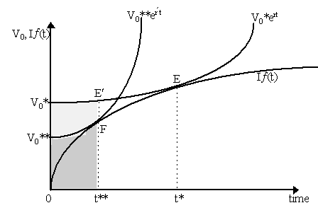
which is the "value" amount of capital. Now we can begin to see the difference between "Real Wicksell Effects" and "Price Wicksell Effects". Examining Figure 3, we see that given a particular r and I¦ (t), we can obtain t* by the standard maximization problem (reaching E by maximizing V0 to V0*). Now, we earlier conjectured that by increasing r, then t* declined. The steps are effectively shown in Figure 3: as interest increases from r to r¢ , then the V0*ert curve swings inside to V0*er¢ t which has the same intercept but a different slope. Of course, it is not feasible given I¦ (t), thus, maximizing with the new interest rate in place, we obtain V0**er¢ t (a shift in the curve downwards) where now the lower intercept V0** is the new value which corresponds to the new maximum, at point F, with the optimal time now reduced to t**.
The question now turns to the amount of capital according to both physical volume (K) and value volume (pK) measures. It seems apparent from Figure 3 that K declines as the area under the curve I¦ (t) below the optimal time is smaller - this is the "Real Wicksell Effect". It is also obvious that pK declines as the area under the corresponding valuation curve (V0* for the first, V0** for the second) will also be smaller - this is the "Price Wicksell Effect". To understand this, recall that at the optimum t (again, normalizing I = 1):
Now, differentiating pK* with respect to t:
but what is dV0/dt exactly? Recall that V0 = ¦ (t)e-rt or ln V0 = ln ¦ (t) - rt so that differentiating the log with respect to t:
and recalling that, at equilibrium ¦ ¢ /¦ = r, then:
Thus, plugging in to our previous equation:
or simply:
Now, the denominator is definitely positive. The numerator is ambiguous. However, recall that ¦ (t) = V0ert. Now, by Taylor's expansion, ert = 1 + rt + (1/2!)(rt)2 + ...., implying that ¦ (t) = V0ert > V0(1+rt). Thus, as dr/dt < 0 from before, then we know that [(1+rt)V - ¦ (t)](dr/dt) > 0 so that the numerator as a whole is positive. Thus, d(pK*)/dt > 0. As dt/dr < 0, then in sum:
Thus, this implies that as t increases, then the "value volume" of capital, pK* increases which, in turn, can be decomposed into "Real" Wicksell effects and "Price" Wicksell effects. The first effect is in the reduction in t and fall in physical volume as r increased to r¢ . The second effect is the portion of the change in which the valuation of pK changed for the same amount of capital. To see the Price Wicksell effect more clearly, examine Figure 4, which is an exaggerated version of Figure 3. The increase in interest from r to r¢ has led to a swivel and shift from V0*ert to V0**er¢ t and thus a change in equilibrium from E (with t*) to F (with t**). The "real" volume of capital under t* is the area under the I¦ (t) curve below t*. The real volume of capital under t** is the smaller area under the I¦ (t) curve below t**. This reduction in area is the Real Wicksell Effect. The Price Wicksell Effect can be noticed by consider the valuation of capital as we moved from t* to t**. In the original case, the value volume of capital, pK was the area under the V0* curve below t*, thus the area formed by 0t*EV0*. After the move, the value volume of capital is the area under the different V0** curve below t**, thus the area 0t**FV0**. Now, consider only the capital from 0 to t**. Obviously, it is the same capital, in physical terms in the original case or after the move as physical capital is measured as the area under I¦ (t) (and thus there is no change). However, in value terms, this same amount of physical capital has a different value volume. Noticeably, after the change, the volume of capital between 0 and t** measured in value terms is captured by the darkly shaded area, i.e. 0t**FV0**. But under the original valuation, this very same physical volume of capital (between 0 and t**) measured in value terms was in fact larger - indeed, it was the area under the V0* curve 0t**E¢ V0*. The lightly shaded area in Figure 4 denoting the difference between the old and the new valuation reflects the "Price Wicksell Effect", i.e. how the change in r and t, by changing valuation V0, has in effect reduced the value volume of capital pK for the same physical amount of capital (between 0 and t**). This is the "Price Wicksell Effect".
What are the implications of this for capital theory? The increase in r has led to a reduction in both the physical volume and the value volume of capital - but by different amounts. Indeed, going the other way (an increase in r and t from t** to t*), it is easy to see that the consequent rise in value volume of capital will be greater than the rise in the physical volume of capital because we have revalued the old capital (between 0 and t*) at a much higher value (the lightly-shaded area). So what? Why not simply consider physical capital and ignore the valuation issue? This, however, is simply not possible. As Wicksell (1901: p.149) points out, capital, in general, is heterogeneous, thus we usually cannot measure them according to technical units. Of course, the same objection lies with labor and land, but it is less forceful for a coalminer can, with enough effort, make a watch and a watchmaker, with much effort, can mine coal - thus we can (try to) index labor according to, say, a "coalminer is worth two watchmakers" or something to that effect. Similarly, an acre of land can be indexed for degrees of fertility, etc. However difficult indexation may be for labor and land, it is virtually impossible to index capital into a homogeneous physical unit because one simply cannot use bottle to make clothes just as much as one cannot use a loom to hold wine - no matter how much we try. As Robinson (1953, 1956) and Lachmann (1956) were to remind us later, it is the "task-specific" nature of capital that creates a far more acute indexation problem than for labor and land. As Wicksell writes "productive capital would have to be distributed into as many categories as there are kinds of tools, machinery and materials, etc., and a unified treatment of the role of capital in production would be impossible" (Wicksell, 1901: p.149). Of course, general equilibrium theory, with its vectors of heterogeneous capital, does not have this difficulty, but then it makes no attempt to derive a rate of return on "capital" but allows each good its own rate of return. However, standard Neoclassical theory relies very much on this. Wicksell's suggestion, following Böhm-Bawerk, is to turn to "time" as the "homogeneous" unit of capital - thus, his efforts with his optimal period of production. When he turns to the possibility of heterogeneity again, and again to the issue of valuation, then we see that the effects come in. We cannot simply use the average period of production to determine the degree of capital-intensity to help determine factor returns, r (and thus w), because the measurement of capital, in value volume terms, itself depends on r and w. As already spotted in Wicksell (1893: p.136-8), we do not know exactly what an increase in r relative to w will do to the degree of capital-intensity. The value volume of capital, like the physical volume, varies inversely with both r and t but part of the change in the value volume is due to this "re-evaluation" of the same physical stock and has nothing to do with changing capital intensity. This, as Robinson notes, "is the key to the whole theory of accumulation and of the determination of wages and profits" (Robinson, 1956: p.396) The most troubling aspect of all this is that the simple marginal productivity theory of distribution, as Wicksell (1901: p.180) emphasizes, may no longer be true. Specifically, recall that pK = [¦ (t) - V0]/r so:
thus differentiating with respect to pK and holding V0 constant:
But recall from before that (dV0/dt) = - t(dr/dt)V0, thus eliminating dt:
so:
or simply:
Since dr/dpK < 0 and since pK > tV0 (by the same logic as before, in a Taylor's expansion, V0e-rt > (1+rt)V0, then if r > 0, then (V0e-rt - V0)/r > tV0. But the term on the left is merely pK, thus pK > tV0). Thus, the entire term on the right is negative, implying then that:
But d¦ (t)/d(pK) is merely the marginal product of capital! Thus, the marginal product of capital is always less than the return on capital. Thus, the marginal productivity theory "is not correct if by "last portion of capital" is meant an increase in social capital" (Wicksell, 1901: p.180). This is the fundamentally disturbing implication of the Price Wicksell Effect.
|
All rights reserved, Gonçalo L. Fonseca
