|
In the "closed" Leontief system, all inputs into production are produced and all outputs exist merely to serve as inputs. Labor requirements, as noted earlier, were "subsumed" in corn requirements via a subsistence wage and thus labor itself became effectively a "produced" good. In the "open" Leontief system, used in Leontief (1941), these assumptions are relaxed and we allow for discretionary consumption and non-produced factors. In other words, there is final consumption demand that has to be met and factor endowments (e.g. labor) that have to be paid. The structure of production must consequently be modified. Let us begin with the open Leontief model without surplus or growth, thus we have a static system. Let us refer to the final demand or consumption of the ith good as Ci. Then, given n goods, we have a n ´ 1 column vector c¢ = [C1, C2, ..., Ci, ..., Cn] representing final demands in the economy. Now, previously we had the output of the jth good being entirely demanded as inputs into other industries. However, now, not all output of good j is demanded as a factor input, but some part of it is demanded for final consumption. Therefore, for the jth industry, we have the condition that:
i.e. output of good j must cover input demands by firms and final demand. Doing so for all industries, j = 1, .., n, we then have the system:
or, in matrix form:
which can be rewritten as:
This can be rewritten as:
which is, as we can see immediately, no longer a homogeneous system of equations. Thus, given a vector of final demands c, we can obtain a determinate solution for x by inversion:
where (I - A¢ )-1 is the inverse of the original technology matrix. However, before we do anything else, we must know for a fact that (I - A¢ )-1 exists, i.e. (I - A¢ ) is non-singular. This can be verified by invoking the Hawkins-Simon conditions. If (I - A¢ ) fulfill the Hawkins-Simon conditions, so that its principal leading minors are positive, then an inverse, (I - A)-1 exists and is non-negative (cf. Nikaido, 1960, 1968; Takayama, 1974). This can in fact be found by using the matrix power series:
This result implies that if (I - A¢ ) fulfills the Hawkins-Simon condition then for any given c ³ 0, there exists an x ³ 0 that solves the system x = A¢ x + c. To understand this, it is worthwhile examining a two-sector case graphically. As we know, with two sectors, the condition (I - A¢ )x = c can be written:
or:
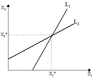
Thus, we have two linear equations. Given C1 and C2, we can draw two lines in a (X1, X2) space (denoted L1 and L2) for the system of equations as in Figure 1. Frontier L1 maps the levels of X1 and X2 that satisfy the first equation and L2 maps the levels which satisfy the second equation. As per the first equation, line L1 has vertical intercept C1/(-a12) < 0, horizontal intercept C1/(1-a11) > 0 and slope (1 - a11)/a12. From the second equation, line L2 has vertical intercept C2/(1-a22) > 0, horizontal intercept C2/(-a21) < 0 and slope a21/(1 - a22) > 0. Thus, the equilibrium values of X1 and X2 which satisfy both equations must be at the intersection of the two locii L1 and L2. This is shown in Figure 1 as the points (X1*, X2*).
It is easy to notice that an intersection is guaranteed only if the slope of L1 is greater than the slope of L2, i.e.
or:
which, it must be noticed, merely states that the determinant of the matrix (I - A¢ ) is positive. This is precisely the Hawkins-Simon condition applied to the two-sector case. If, on the other hand, |I - A| < 0, then notice that this would imply that (1-a11)/a12 < a21/(1-a22) so that the slope of L1 would be smaller than the slope of L2 which, as we can immediately see diagramatically, implies that L1 and L2 will not intersect - i.e. there is no non-negative solution X1*, X2*. Finally, let us note that the intercepts of the locii contain C1 and C2 in them - thus a rise in C1 will obviously shift the locus L1 to the right whereas a rise in C2 will shift the locus L2 to the left. Thus, rises in either C1 or C2 or both will lead to rises in both equilibrium X1* and X2*. Similarly, a fall in the own demand (i.e. a fall in a11 or a22 coefficients) will result in lower equilibrium outputs whereas a fall in cross-demand (a12 and a21) will result also in lower equilibrium outputs. This can be observed from the slope and intercept conditions. Let us now turn to the dual problem - namely, prices. We have assumed no surplus, thus we now must ask where the "final demand" in the quantity side arises from. The simplest explanation would be to presume that there are primary inputs which receive returns which they then use to make final demands on output. A "primary input" is a non-produced factor of production - for instance, land or labor. An example, would be workers who sell their labor to firms for a wage and, from the proceeds, demand consumption goods. In this case, let a0j be the amount of labor necessary to produce a unit of good j. Let workers receive a uniform wage rate, w. Thus, for production to be viable, the sale price of good j must not fall below the cost of producing a single unit of good j:
So, sale price must cover unit costs of purchasing inputs from other firms and paying labor its wages. As there is no surplus, we can assume an equality for this and all other sectors, so:
is our system of equations, or in matrix form:
or, thinking of a0 = [a01, ..., a0n]¢ as a column vector of unit labor requirements, then:
We can rewrite this as:
which is also a non-homogeneous system. Thus a solution p can be found by inversion, namely:
The existence of the inverse (I - A)-1 is effectively solved by the same manner as before. If the Hawkins-Simon conditions are fulfilled for (I - A¢ ), they will also be fulfilled for (I - A), and thus an inverse will exist and will be non-negative. Thus for any given non-negative set of unit wage-bills, wa0 ³ 0, there is a set of non-negative prices p ³ 0 which solve the system p = Ap + wa0. A diagrammatic example demonstrating the necessity of the Hawkins-Simon conditions for the existence of a solution p can also be drawn for the two-sector case and will be analogous to before. Namely, taking the two-sector model, then (I - A)p = wa0
or:
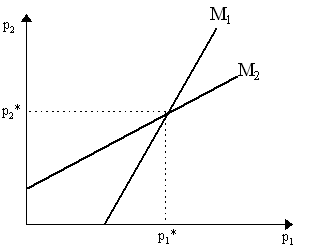
We can thus depict these two equations as in Figure 2 via the lines M1 and M2. The line M1 represents the levels of prices which fulfill the first equation, thus it has vertical intercept wa01/(-a21) < 0, horizontal intercept wa01/(1-a11) > 0 and slope (1-a11)/a21 > 0. Similarly, M2 represents the values fulfilling the second equation, thus it has vertical intercept wa02/(1-a22) > 0, horizontal intercept wa02/(-a12) < 0 and slope a12/(1-a22) > 0. The solution values p1* and p2* are given by the intersection of the two curve M1 and M2. Notice that if the primary factor payments increase, then M1 and M2 shift accordingly. Specifically, if w increases, M1 shifts to the right and M2 shifts to the left. A rise in labor input requirements, a01 and a02 will have analogous effects. The necessity of the Hawkins-Simon conditions for the existence of a non-negative p1*, p2* can be noted by referring to the fact that M1 must have a greater slope than M2, i.e. that (1-a11)/a21 > a12/(1-a22), which translates simply into (1-a11)(1-a22) - a21a12 > 0.
Luigi Pasinetti (1975) sees the condition that p = (I - A)-1wa0 as insinuating the Classical "labor theory of value". If w = 1, we can see that (I - A)-1a0 is a vector of vertically integrated labor coefficients which "represents the quantities of labor directly and indirectly "embodied" in each physical unit of the commodities of the net product of the economic system (what Marx called "values" by definition)" (Pasinetti, 1975: p.76). Thus, prices p are proportional to the physical quantities of embodied labor - the essence of the labor theory of value. Of course, we need not assume that labor is the only primary input. We could have several primary inputs at once. For instance, suppose we have m primary inputs, letting bkj denote the unit input coefficient of primary input k into the production of the jth output. Each primary input receives a return wk and thus, for the jth output, the price-cost equality becomes:
so that we obtain a system of equations in the following form:
where w is a (m ´ 1) column vector of primary input returns and B is an (n ´ m) matrix of unit input coefficients for the primary factors. Assuming w and B are given, then we can solve this for p by inversion again:
which again, is determinate by the Hawkins-Simon conditions.
|
All rights reserved, Gonçalo L. Fonseca


