|
________________________________________________________
________________________________________________________ Contents (1) Introduction In the Harrod-Domar growth model, steady-state growth was unstable. In the popular term of the day, it was a "knife-edge" in the sense that any deviation from that path would result in a further move away from that path. However, Robert M. Solow (1956), Trevor Swan (1956) and, a bit later, James E. Meade (1961) contested this conclusion. They claimed that the capital-output ratio of the Harrod-Domar model should not be regarded as exogenous. In fact, they proposed a growth model where the capital-output ratio, v, was precisely the adjusting variable that would lead a system back to its steady-state growth path, i.e. that v would move to bring s/v into equality with the natural rate of growth (n). The resulting model has become famously known as the "Solow-Swan" or simply the "Neoclassical" growth model. A brief word or two on historical precedence is warranted. James Tobin (1955) introduced a growth model similar to Solow-Swan which also included money (and thus a predecessor of the monetary growth theory). However, Tobin did not solve explicitly for the stability of the steady-state. Also, it is become increasingly common to credit Jan Tinbergen (1942) as presenting effectively the same model as Solow-Swan, including even empirical estimates of the relevant coefficients. Finally, Harold Pilvin (1953), before Solow, had argued that the Harrodian knife-edge problem could be resolved if a flexible capital-output ratio were introduced, but he did not formulate the concept of a steady-state. Harrod's (1953) response to Pilvin is quite instructive in stressing that flexible technology does not, in fact, resolve the Harrodian knife-edge as he originally conceived it. But more on this later. (2) The Solow-Swan Growth Model For the analysis, let us begin with the macroeconomic equilibrium condition that aggregate demand equal aggregate supply, Yd = Y. This translates, automatically, into claiming that investment equals savings, i.e. I = S. Now, according to the simplest of consumption functions, C = cY, where c is the marginal propensity to consume. Now, by definition, savings are S = Y - C = Y - cY or simply S = (1-c)Y. Letting s = (1-c), the marginal propensity to save, then we can express savings as some proportion of total output,
so combining this with the macroeconomic equilibrium condition:
Dividing through by L, the amount of labor in the economy, then:
so, letting i = I/L and y = Y/L, we see that the macroeconomic equilibrium condition becomes:
Now, aggregate supply (output) is given by a production function of the general form:
which is assumed to vary continuously with K and L (i.e. smooth substitutability) and exhibits constant returns to scale. Dividing through by L:
or, letting k = K/L, we can rewrite this as:
where ¦ (·) is the "intensive" or "per capita" form of the production function F(·). As a result, the macroeconomic equilibrium condition can be rewritten as:
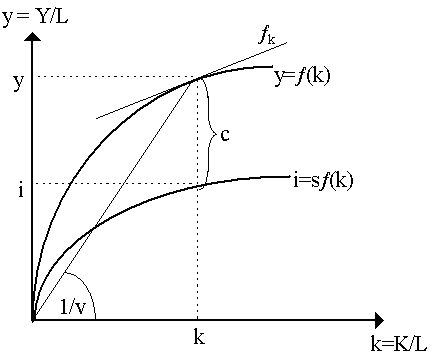
This can be thought as representing equilibrium investment per person. If we assume that macroeconomic equilibrium holds at all times (i.e. I = S always), then i = s¦ (k) can also be referred to as the actual investment per person. Figure 1 depicts the intensive production function y = ¦ (k) and the actual (equilibrium) investment function, i = s¦ (k). Notice that at any k, we can derive investment per person, i, output per person, y, and, residually, consumption per person (c = C/L = y - i). The slope of the intensive production function is ¦ k = ¶ ¦ (k)/¶ k which happens to also be the marginal product of capital, i.e. ¦ k = FK (see our discussion of intensive production functions). Finally, notice that the capital-output ratio, v = K/Y = k/y, is captured as the slope of a ray from the origin to production function. Thus, changing k will change the ray and thus v. So, unlike the Harrod-Domar model, v is not exogenously fixed.
So, let us turn to growth. By assumption, we assume population grows exogenously at the rate n, i.e.
If there is no investment, then k = K/L will automatically fall as population grows. So, for k to be constant, there must be investment (i.e. capital must grow) at rate n:
where we have attached the superscript "r" to indicate that this is the required growth rate of capital to keep the capital-labor ratio, k, steady. As investment is defined as I = dK/dt, then we can rewrite this as:
where Ir is required investment. Dividing through by labor, L, Ir/L = nK/L, or:
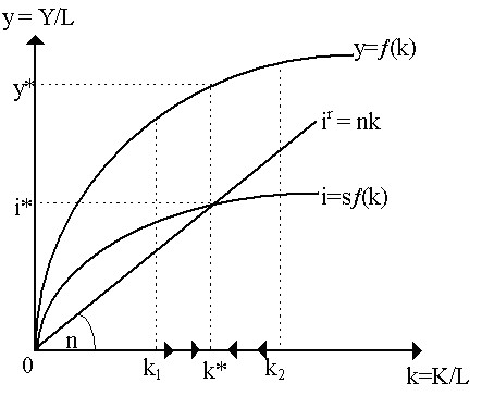
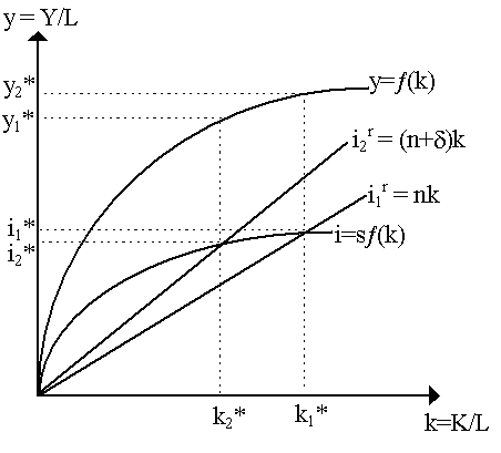
which is the required investment per person to maintain a steady k. Why are we obsessed with keeping k constant? Well, we are interested in "steady-state" growth which, as defined by Gustav Cassel (1918), means "proportional" growth in a manner that there are no induced changes in relative prices over time. It is obvious (from Figure 1, for instance) that a change in k will change the marginal products of capital and labor. Assuming the marginal productivity theory of distribution holds, so that capital and labor are, in equilibrium, priced at their marginal products, then if we allow k to change over time in our solution, then we are also allowing relative factor prices to fluctuate over time. As Cassel's definition of a "steady-state" growth equilibrium does not allow this, then, consequently, we must focus on getting k to stay constant. We can depict the steady-state k in Figure 2, by superimposing the required investment function, ir = nk, on top of our old diagram. Notice that only at k* is actual investment equal to required investment, i = ir. At any other k, i ¹ ir.
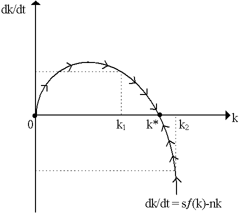
It is a simple matter to note that not only is k* our steady-state capital-labor ratio, it is also a stable capital-labor ratio. If our initial capital labor ratio is below k* (e.g. at k1), then actual investment is greater than required investment, i > ir, which means that capital is actually growing faster than labor, so k will increase. Conversely, if our initial k is above k* (e.g. at k2), then actual investment is below required, i < ir, so capital is growing slower than labor, so k will fall. Thus, the steady-state capital-labor ratio, k*, is stable in the sense that any other k will have the tendency to approach it over time. We can capture the entire stability story in terms of a simple differential equation as follows:
or, plugging in our terms for i and ir:
which is the fundamental Solowian growth equation. At steady-state, k*, dk/dt = 0 and so (ignoring the trivial origin case), it must be that s¦ (k*) = nk*, i.e. k* is the steady-state. In Figure 3, we depict the phase diagram of the Solowian differential equation. Notice that dk/dt = 0 at steady-state k*. If we are at k1 < k*, then dk/dt > 0, whereas at k2 > k*, then dk/dt < 0. [Note: if we start at the origin, k = 0, equilibrium holds trivially (i = ir = 0). However, we can ignore the origin solution safely, not only because it is not very interesting but also because it is unstable, i.e. if k > 0, then the underlying dynamics drive us away from the origin].
(3) Adding Depreciation Before proceeding, let us insert a slight modification in the model to account for capital depreciation. The macroeconomic equilibrium condition (i = s¦ (k)) remains the same; it is the required investment rate that now becomes different. In order for k to remain constant, then capital must grow not only to accompany population growth but also to cover depreciation of old capital. Specifically, we now have:
as our required investment rate, where d is the capital depreciation rate. The fundamental Solowian differential equation needs to be rewritten as:
In terms of Figure 2, all that will happen when we insert capital depreciation is that the required investment line ir will become steeper (with slope n+d ) and so the steady-state ratio k* will be lower (see Figure 4). However, notice that now the growth rates of the level variables -- capital stock, output and consumption -- all rise to (n+d).
|
All rights reserved, Gonçalo L. Fonseca
