One of the main drawbacks of the "preference is a preference" defense of discounting was that it was not clear that this is so. If positive time-preference is to be introduced as an expression of people's natural tastes, it must be introduced as an axiom of preference itself or derived from more primitive axioms. Yet impatience is a general behavioral postulate. We are not talking about preferences over toothpastes which can vary immensely across people; we are referring to a time-discount factor that is positive and present, to a greater or lesser degree, in everybody. It has a generality and universality of applicability. To say that it "just a preference" does not explain its regularity. The derivation of "impatience" from more basic axioms on preferences were attempted by Kelvin Lancaster (1963), Tjalling Koopmans (1960, 1972), Koopmans, Diamond and Williamson (1964), Peter Diamond (1965) and Peter Fishburn and Ariel Rubinstein (1982). Here we shall consider Koopmans's contributions, which were directly concerned with deriving a discount factor from the social planner's utility. This turns out to be a quite subtle and profound defense of discounting. Koopmans's (1960) inspiration was John von Neumann and Oskar Morgenstern's (1944) trick with choice under uncertainty. Recall that they stipulated that people have preferences over lotteries and then found the necessary axioms on these preferences that would yield Bernoulli's "expected utility" form. Similarly, Koopmans argued that the social planner has preferences over infinite consumption paths and then searched for the axioms that would make such preferences representable by a Samuelson intertemporal utility function with discounting. Intuitively, letting S(·) represent the social planner's utility function over consumption paths, then, for any two path C and C¢, Koopmans (1960) sought to find axioms on S(·) such that:
where U(·) is an elementary, single-generation utility function and b is a time-discount factor. So, rather than creating a social welfare function by adding up each generation's utility, Koopmans goes the other way and derives generational utility functions U(·) plus discount factor b from the planner's social welfare function S(·). Notice there was a second purpose to Koopmans's construction: namely, the restoration of ordinality into the intertemporal utility construction. Obviously, if we take the Samuelson function, å t=0¥ bt U(Ct), as our social welfare function, then it is a cardinal function: the particular numerical values we give our realized generational utilities, U(Ct), U(Ct+1), etc. matter very much as they will be subsequently added up. But like von Neumann-Morgenstern, Koopmans was aiming at a "ordinal utility which is cardinal". The real and only utility function in the Koopmans world is S(·) and it is defined as a representation of social planner's preferences over infinite-horizon consumption paths. This utility function S(·) is ordinal, i.e. the numerical values we assign to S(C), S(C¢ ), etc. do not matter, as long as the preference ordering over paths is maintained. So, in this way, Koopmans makes the whole intertemporal utility exercise "acceptable" to radical Paretians. Koopmans (1960) proceeded as follows. Let C denote an entire infinite-horizon consumption path and Ct denote the tth element of that path, so C = {C1, C2, C3, .., Ct, ...}. We will let the term 2C denote the path C excluding the first entry, i.e. 2C = {C2, C3, C4, ..., Ct, ..,}. Thus, the path C can be written as C = {C1, 2C}. Let D denote the "commodity space", in this case the set of infinite-horizon consumption paths, so C Î D . It is assumed that the social planner's preferences can be captured by a nice social utility function S: D ® R, where if S(C) ³ S(C¢ ), then the social planner prefers path C to path C¢ . Koopmans then imposes the following axioms (he calls them "postulates") on S(·):
Note that axioms (P.1)-(P.5) are assumed directly on the social planner's utility function S: D ® R -- which is assumed to exist and somehow represent the planner's "preferences" over intertemporal allocations. Of course, we should say something about whether the social utility function S represents these preferences, and how these utility postulates might be connected to other, more primitive axioms on preferences. Koopmans (1972) forges this connection, but we shall skip it here. The meaning of the axioms can be briefly explained. Postulate (P.1) is a simple continuity axiom: any slight variation in the path does not lead to drastic changes in the social planner's utility. It is expressed in this funny way for technical reasons. Axiom (P.2) means that every generation counts, i.e. if there are two paths that are identical in every respect except for the first period where it is drastically different, then the social welfare of those paths will be different. Postulate (P.3) is a kind of independence axiom. Specifically, it argues that if two paths are identical except in one period, then it does not matter what the identical part looks like when comparing them. There is non-complementarity between periods in the sense that the social planner's preference over what generation t achieves is independent of his preferences over what generation t+1 achieves. Axiom (4), stationarity, is the famous and most debatable one in the Koopmans array. What it says explicitly is that preferences between two events remain the same, even if we push these events forward. For instance, consider the baseline consumption path (1, 1, 1, 1..., ), so there is steady consumption of one unit of the consumption good every period. Now suppose that the following adjustments are possible. Namely, we can either add X to the first time period or add amount Y to the second time period, so that the two alternative paths are now: C = (1 + X, 1, 1, 1, ...) or C¢ = (1, 1 + Y, 1, 1, ....). Suppose that the social planner's preferences are such that:
he prefers the X adjustment today rather than the Y adjustment tomorrow. Now, suppose we push the event forward by a period, and construct path D = (1, 1+X, 1, 1, ...) and path D¢ = (1, 1, 1+Y, 1, ...). Notice that D = (1, C) and D¢ = (1, C¢ ), so all we have done is shunted each of the "events" forward by one period. Stationarity says that if S(C) > S(C¢ ) then it must be that S(D) > S(D¢ ), i.e.
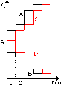
and vice-versa. So, what the stationarity axiom effectively says is that intertemporal preferences between two periods remain the same even if we shunt those two periods further ahead in time. Intuitively, if the social planner prefers one apple today to two apples tomorrow then he will prefer one apple in 30 days to two apples in 31 days. Interestingly, Diamond (1965) attempted to redo this analysis without the stationarity axiom. Koopmans (1960) shows that a social welfare function which possesses these five axioms will necessarily exhibit positive time preference. We shall not attempt to prove this here. But we can give an idea of why this is so with an example. Suppose there are four utility paths A, B, C and D, as depicted in Figure 1 (A and B are black, C and D are red). Let us suppose that the consumption path A is superior to consumption path B every step of the way, so, socially, S(A) > S(B). Now, suppose that paths C and D are constructed in the following manner. For the first period (t = 1), path C maintains consumption level c0, but subsequently, for t = 2, 3, 4, .. it follows precisely the same path A did. Thus, C is merely A with a one-period lag. Similarly, D keeps consumption c0 for the first period and follows path B with a one-period lag thereafter. Thus, C = {c0, A} and D = {c0, B}.
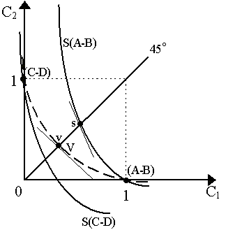
As far as the first period is concerned, paths C and D are identical and only thereafter does the difference begin. Obviously, then, S(C) > S(D) for the same reasons that S(A) > S(B). In fact, it is a straightforward application of the stationarity axiom. But what about the utility difference? Intuitively, the utility difference between C and D should be less than the utility difference between A and B because for a little while (i.e. during period t = 1), paths C and D yield the same consumption and thus utility. Because paths C and D are less different than paths A and B, their utility difference should be smaller. Heuristically, then, S(A - B) > S(C - D). This is what Koopmans, Diamond and Williamson (1964) labelled "time perspective" in the sense that the difference between utility streams is smaller the further away in time it is.. The necessity of time preference follows from this observation. Suppose, for example, that A = {3, 3, 3, ..., } and B = {2, 3, 3, 3....}, so (A - B) = {1, 0, 0, 0, ...}. At the same time, C = {c0, 3, 3, 3, ...} and D = {c0, 2, 3, 3, ...} so (C - D) = {0, 1, 0, 0, ...}. Then obviously the statement S(A-B) > S(C - D) implies that S(1, 0, 0, ...) > S(0, 1, 0, 0, ..). This is time preference. To see this explicitly, notice that from the third period onwards, (A-B) and (C-D) are identical. Let us just lop of all the remaining periods except the first two from consideration and so consider the plot in a simple indifference map (Figure 2). Now, by the non-complementarity axiom, S(A-B) > S(C - D) implies that {1, 0} is preferred to {0, 1}. In Figure 3, this translates into saying that the social indifference curve S(A-B) which passes through (1, 0) lies above the social indifference curve S(C - D) which passes through (0, 1).
The social indifference curves in Figure 2 exhibit time preference. We can deduce this by comparing indifference curve S(A-B) with an alternative indifference curve V. Notice that V (dashed curve in Figure 2) passes through both (1, 0) and (0, 1). We see then that V is an indifference curve which has no time preference -- it is indifferent between (1, 0) and (0, 1). Now, let us assume that S and V are additively separable. This means that we can decompose the utility of consuming bundle (C1, C2) into two utility components, i.e.
where S1, S2 are the utilities of consuming in periods 1 and 2 respectively for the social utility function S while V1, V2 are the corresponding utilities for social utility function V. Now, let s and v denote the points where S and V intersect the 45° line (cf. Figure 2). As these are on the 45° line, then, for simplicity and abusing notation a bit, let s = [s, s] and v = [v, v]. Notice also that s = a v, where a is a positive scalar. The slope of the indifference curves S and V at the 45° lines are captured by the marginal rates of substitution:
But notice, in Figure 2, that S at the 45° line is steeper than V at the 45° line. Thus:
But as MRSV(v) = 1, then it must be that MRSS(s) > 1, or S1¢ (s) > S2¢ (s). In English, if we are consuming the same amount in both periods, we would make a gain in utility by reallocating a unit of consumption from period 2 to period 1, i.e. the present is "preferred", in pure utility terms, to the future. Notice that the arguments in the indifference curve S are identical because we are evaluating it on the 45° line. So the difference between S1¢ (s) and S2¢ (s) must arise purely from the difference in the utility parts, S1(·) and S2(·), and not in the amounts consumed. There is pure time preference. By the Archimedean property of numbers, there is some factor b Î [0, 1] such that b S1¢ (·) = S2¢ (·). So, our social utility function can be rewritten as
or defining S1(·) = U(·):
Thus, we have decomposed our social welfare function into a single elementary utility function U(·) and a discount factor b . We can proceed by iterative construction to show that:
i.e. our social planner's utility function defined over an infinite horizon is identical to the Samuelson (1937) discounted intertemporal social welfare function. The pure rate of time preference, call it r , can be defined as r = (1-b )/b , implying that:
so, as long as r > 0, then b < 1. If r = 0 (no time preference rate), then b = 1 (no time discount factor). Let us step back and think about what we have just done. A positive time preference rate on the social planner's utility has been deduced (with the assistance of additive separability) from the simple observation of the property of "time perspective", i.e. that S(A - B) > S(C - D). This assertion was purely intuitive: C and D share the first time period, so C should be "less different" from D than A is from B. This, in a nutshell, is the crux of the argument. What exactly makes it work? Critical in this intuition is the sensitivity axiom (P.2). The implications of this axiom can be thought through as follows. Suppose that a consumption path can be permanently improved forever if we merely starve the first generation to death. In the grand scheme of things -- i.e. in an infinite horizon -- the utility loss of the generation in the first period seems to be negligible when compared to the increased utility of all the remaining generations. What Koopmans was seeking with his sensitivity axiom was to prevent the social planner from making such a calculation. He should not ignore the utility loss of one generation just because it is one period out of infinity. Sensitivity is thus not merely a mathematical condition, it is also an "ethical" condition. We begin the see how "sensitivity" is related to the time perspective property. In our simple example, if we could ignore the first period, then the difference between paths A and B could be considered identical to the difference between paths C and D. But, by sensitivity, we cannot ignore the first period. The fact that C and D share the same consumption in the first period must be accounted for in the social planner's preferences. It is from this assertion that we can conclude that S(A - B) > S(C - D) and, as we have seen, thereafter go all the way to positive time preference and representation of the planner's social utility by a Samuelson function. For details, consult Koopmans, Diamond and Williamson (1964). There is an observation worth making at this point. Koopmans's analysis suggests that if we attempt to derive a social welfare function without time preference, then we are implicitly violating sensitivity somehow. This makes sense. Without time preference, the utilities achieved by any finite number of generations can be "ignored" as the remaining infinity overwhelms them completely. Indeed, in continuous time, such negligibility is automatic. But it is the ethical implications of this that are interesting. What Koopmans has highlighted with his exercise is the interlinkage between sensitivity with time preference. On the one hand, discounting is unethical because, say, it could be used to justify current environmentally-destructive activities whose effects would only be felt millions of years in the future. On the other hand, discounting is ethical because without it, the infinite future overwhelms the finite present. More acutely, without discounting, we could justify savagely destroying one generation now if it yielded a series of minuscule gains (no matter how small) that would accrue forever after. An ethical balance must be struck: either we count every generation equally (in which case, no single generation counts at all), or we allow discounting (in which case every generation counts, but some less than others). Which is more ethical? See Kenneth Arrow (1979) for some reflections on this.
|

All rights reserved, Gonçalo L. Fonseca