|
________________________________________________________
________________________________________________________ Contents (A) The Production Function (A) The Production Function Let us begin with the production function, a function summarizing the process of conversion of factors into a particular commodity. We might propose a production function for a good y of the following general form, first proposed by Philip Wicksteed (1894):
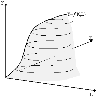
which relates a single output y to a series of factors of production x1, x2, ..., xm. Note that in writing production functions in this form, we are excluding joint production, i.e. that a particular process of production yields more than one output (e.g. the production of wheat grain often yields a co-product, straw; the production of omelettes yields the co-product broken egg shells). Using Ragnar Frisch's (1965) terms, we are concentrating on "single-ware" rather than "multi-ware" production. For heuristic purposes, the production technology for the one-output/two-inputs case is (imperfectly) depicted in Figure 2.1. Output (Y) is measured on the vertical axis. The two inputs, which we call L and K which, for mnemonic purposes, can be called labor and capital, , are depicted on the horizontal axes. We ought to now warn that henceforth, throughout all our sections on the theory of production, all capital is assumed to be endowed, i.e. there are no produced means of production. The hill-shaped structure depicted in Figure 2.1 is the production set. Notice that it includes all the area on the surface and in the interior of the hill. The production set is essentially the set of technically feasible combinations of output Y and inputs, K and L.
A production decision -- a feasible choice of inputs and output - is a particular point on or in this "hill". It will be "on" the hill if it is technically efficient and "in" the hill if it is technically inefficient. Properly speaking, the production function Y = ¦ (K, L) is only the surface (and not the interior) of the hill, and thus denotes the set of technologically efficient points of the production set (i.e. for a given configuration of inputs, K, L, output Y is the maximum feasible output). Obviously, the hill-shape of the production function indicates that the more we use of the factors, the greater output is going to be (at least up to the some maximum, the "top" of the hill). The round contours along the production hill can be thought of as topographic contours as seen on maps and will serve as isoquants in our later analysis. The slope of the hill viewed from the origin captures the notion of returns to scale. Throughout the next few sections, we shall be outlining the technical properties of the production function. The representation of production functions in the diagrammatic form of "hills" and the corresponding analysis of production theory in terms of isoquant contours, etc. was initiated by Vilfredo Pareto (1906) and much of the analysis of its technical properties was largely advanced by the "Paretian" school of Hotelling, Frisch, Samuelson, Hicks, Shephard, etc. between the 1930s and the 1950s. In the 1950s, the Neo-Walrasians (e.g. Koopmans, 1951; Debreu, 1959) approached the analysis of the technical properties of production in a somewhat different spirit. Specifically, instead of focusing on the "production function" and its derivatives as the Paretians had done, the Neo-Walrasians preferred to analyze it via vector space methods and convex analysis. On a more formal note, we should outline the properties of the production function, as normally assumed by Neoclassical economists. Let there be m factors of production and let vector x = (x1, x2, .., xm) denote a bundle of factor inputs. We shall define an input space as the acceptable set of inputs for our economy. Commonly, a bundle of factor inputs x is deemed "acceptable" if every entry in that vector, i.e. the quantity of every factor, is a non-negative, finite real number. Thus, any input bundle x lies in R+m, the non-negative orthant of m-dimensional Euclidian space. Thus, R+m is our input space. Let y be output, which is assumed to be a single, finite number, i.e. y Î R. Thus, a production function ¦ maps acceptable input bundles to output values, i.e. ¦: R+m ® R. More specifically, ¦(x) is the maximum output achievable for a given set of acceptable inputs, x Î R+m. The following assumptions are often imposed on any generic production function ¦ : R+m ® R
These assumptions will be clarified as we go on. For the moment, let us just make the following notes. Assumption (A.1) simply defines the production function as a well-defined function of inputs ¦ : R+m ® R. Nothing new there. Assumption (A.2) simply establishes that one cannot produce something from nothing. This is somewhat self-evident, at least for economists. Obviously, in other walks of life, one can produce something without inputs (e.g. "nice thoughts" can just be, well, "thought up" without inputs), but most examples of these things are outside the realm of economics. The monotonicity assumption (A.3) is also straightforward: increasing inputs leads to an increase in output (or, more precisely, no decrease in output). Although common, we will have more to say on this later. Assumption (A.4) is made largely for mathematical ease; later on, we shall relax this assumption somewhat. Assumption (A.5), the quasi-concavity of the production function ¦ , is the more interesting one. We shall have much more to say on this later. Finally, (A.6) is imposed as a mathematical necessity. The assumptions given earlier imply that, for any given production function y = ¦ (x1, x2, .., xm), it is a generally the case that, at least up to some maximum point:
for all factor inputs i = 1, 2, ..., m. In other words, adding more units of any factor input will increase output (or at least not reduce it). This is the heart of assumption (A.3). However, it is also common in Neoclassical theory to also impose (A.5), i.e. to assume "quasi-concavity" of the production function. It is often the case in economics that the quasi-concavity assumption implies that:
for all i = 1, .., m, i.e. diminishing marginal productivity of ith factor. It is worthwhile to spend a few moments on the diminishing marginal productivity assumption. This means more we add of a particular factor input, all others factors remaining constant, the less the employment of an additional unit of that factor input contributes to output as a whole. This concept performs the same function in production functions as diminishing marginal utility did in utility functions. Conceptually, however, they are quite distinct. (i) The Law of Diminishing Returns The idea of diminishing marginal productivity was simultaneously introduced for applications of factors to a fixed plot of land by T.R. Malthus (1815), Robert Torrens (1815), Edward West (1815) and David Ricardo (1815). It was applied more generally to other factors of production by proto-marginalists such as J.H. von Thünen (1826), Mountiford Longfield (1834) and Heinrich Mangoldt (1863). The apotheosis of the concept is found in the work of John Bates Clark (1889, 1891, 1899) and, more precisely, in Philip H. Wicksteed (1894). It was originally called the "Law of Diminishing Returns", although in order to keep this distinct from the idea of decreasing returns to scale, we shall refer to it henceforth as the "Law of Diminshing Marginal Productivity" Let us first be clear about the definition of the marginal productivity of a factor. Letting Dxi denote a unit increase in factor xi, then the marginal product of that factor is Dy/Dxi, i.e. the change in output arising from an increase in factor i by a unit. Mathematically, however, it is more convenient to assume that D x is infinitesimal. This permits us to express the marginal product of the factor xi as the first partial derivative of the production function with respect to that factor -- thus the marginal product of the ith factor is simply ¶y/¶xi = ¦i. If we do not wish to assume that factor units are infinitely divisible or if we do not assume that the production function is differentiable, we cannot express the marginal product mathematically as a derivative. [We should note that both Carl Menger (1871) and John A. Hobson (1900, 1911) defined "marginal product" differently: rather than being the output gained by an enterprise from the addition of a factor unit, Hobson defined it as the output lost by the enterprise by the withdrawl of a factor unit. This caused a problem for the "adding up" issue in the marginal productivity theory of distribution, although, as was clarified later, when marginal product is not defined so discretely, it does not make a difference which measure we use. For a useful discussion of the dilemma involving the measurement of the "marginal unit", see the discussion in Fritz Machlup (1937). Finally, we must note that a far more novel and interesting definition of marginal productivity was introduced by Joseph M. Ostroy (1980, 1984) where the concept is redefined in terms of contributions to tradeable surpluses, and thus both widened and deepened in scope.] However, assuming marginal products exist and are well defined, then why diminishing? Taking Clark's famous analogy:
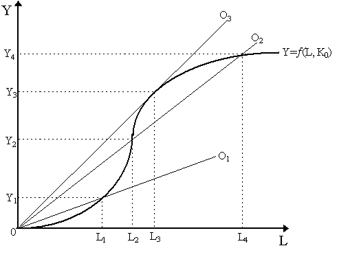
The implication, then, is that as we increase the amount of labor applied to a particular fixed amount of land, each additional unit will increase total output but by smaller and smaller increments. When the field is empty, the first laborer has absolutely free range and produces as much as his body can reasonably do, say ten bushels of corn. When you add a second laborer to the same field, total output may increase, say to eighteen bushels of corn. Thus, the marginal product is eight. Why? The basic idea is that by adding the second man, the field gets "crowded" and the men begin to get in each other's way. If that explanation does not seem credible, think of the units of labor in terms of labor-hours for a single man: in the first hour, a particular man produces ten; in the second hour he produces eight, etc. The diminution can be explained in this case as an "exhaustion" effect. Taking another example, suppose we apply a man to a set of shoe-making tools and a given swathe of leather; let us say he can produce ten pairs of shoes in a day. Add a second man to this without adding more shoe-making tools or increasing the leather, and one can easily envisage that more shoes get made in a day, but that the work of the shoe-makers slows down as they pick up the same tools in an alternating sequence of turns and perhaps fight over them a bit. For other factors, different stories are told. In Ricardo's original story, the land is subject to diminishing marginal returns because of the assumption that land has different degrees of fertility and the most fertile acres are used first, and the less fertile ones added later. We can conceive this more simply in that increasing the amount of land without increasing the amount of labor that works on it will lead to less output per worker. However it is justified, many Neoclassical theorists basically accept diminishing marginal productivity as an axiom - "the diminishing marginal productivity of labor, when it is used in connection with a fixed amount of capital, is a universal phenomenon. This fact shows itself in any economy, primitive or social." (Clark, 1899: p.49). However much early economists tried to claim it to be a natural law, this "axiom" turns out to be closer to a rather debatable assumption (cf. Karl Menger, 1954). Nonetheless, it is important to clearly note a few matters in relation to this. Firstly, the idea that marginal product is always diminishing can be disputed (and will be disputed). Francis A. Walker (1891) took J.B. Clark to task for not recognizing the possibility of increasing marginal productivity (albeit, see Clark (1899: p.164)). Secondly, as Pareto (1896, 1902) was quick to point out, it is not always true that if one adds a unit of a factor to an existing production process, output will increase. "If a pit has to be dug, the addition of one more man will make little difference to the day's output unless you give the man a spade" (Cassel, 1918: p.179). This difficulty is even more clear if we see the problem in terms of the marginal product of capital: if a pit has to be dug, the addition of one more spade will make no difference to output unless you add a man to use it. Thus, one must be very careful when pronouncing the idea of marginal productivity since we may need to produce in fixed, constant factor proportions. Thirdly, it is important to underline that the marginal product is not, properly speaking, the contribution of the marginal unit by itself. Some commentators (e.g. E.v. Böhm-Bawerk, 19??; cf. Robertson, 1931) seem to have gone on to make arguments that seem to imply, in the context of our example, that the second man produces eight bushels of corn. Of course, this is not necessarily true. The second man may very well produce nine or ten or eleven and still the total output increases only to eighteen because the first man reduces his output to nine, or eight or seven in the presence of the second. In our example, output increases from ten bushels to eighteen bushels when one adds the second man not because the second man only adds eight, but rather because his presence on the field makes the situation such that the total output of both men is eighteen. Notice that the contribution per man is reduced: the average product is actually nine. This may very well be how much each of the two laborers contributes. But this is not what interests us: what we wish to note is that by adding the second man, output was increased by eight. Thus, the marginal product of the second man is eight. But his actual contribution may be very different than this. Finally, and above everything, it is very important to note that in deriving the marginal product of a factor, we are holding all other factors fixed. Specifically, in our earlier example, labor varied and land (and indeed all other factors) was fixed. Thus, diminishing marginal productivity has nothing to do with "returns to scale", i.e. the increase in output when we increase all factors. If we increased both land and labor in our example, then there might very well be no reduction in output per man (indeed, there is actually no reason for it, but we shall return to this later). (ii) The Law of Variable Proportions Marginal productivity is not obvious in the production function Y = ¦ (L, K) in Figure 2.1 as both inputs are varying there. We must first fix one of the factors and let the other factor vary. This is shown in Figure 2.2, by the "reduced" production function Y = ¦ (L, K0), where only labor (L) varies while capital is held fixed at K0. To obtain this from the former, we must figuratively "slice" the hill in Figure 2.1 vertically at the level K0. Thus, Figure 2.2, which represents the reduced production function Y = ¦ (L, K0), is a vertical section of the hill in Figure 2.1. A reduced production function where all factors but one are held constant are often referred to as the "total product" curve.
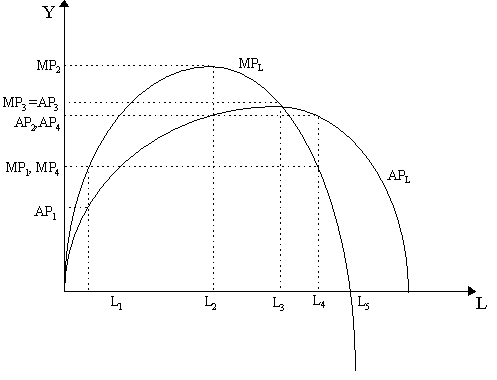
The total product curve in Figure 2.2 can be read in conjunction with the average and marginal product curves in Figure 2.3. The total product curve is originally due to Frank H. Knight (1921: p.100), and much of the subsequent analysis is due to him and John M. Cassels (1936). Although both these sets of curves have long been implicit in much earlier discussions (e.g. Edgeworth, 1911), average and marginal products were confused by early Neoclassicals with surprising frequency. The particular shape of the total product curve shown in Figure 2.2 exhibits what has been baptized by John M. Cassels (1936) as the Law of Variable Proportions -- effectively what Ragnar Frisch (1965: p.120) quirkily renamed the ultra-passum law of production. The marginal product of the factor L is given by the slope of the total product curve, thus MPL = ¶ Y/¶ L = d¦ (L, K0)/dL. As we see, at low levels of L up to L2 in Figure 2.2, we have rising marginal productivity of the factor. At levels of L above L2 we have diminishing marginal productivity of that factor. Thus, marginal productivity of L reaches its maximum at L2. We can thus trace out a marginal product of L curve, MPL, in Figure 2.3. The labels there correspond to those of Figure 2.2. Thus the MPL curve in Figure 2.3 rises until the inflection point L2, and falls after it. It becomes negative after L5 - which would be equivalent to the "top" of the reduced production function, what Frisch (1965: p.89) calls a "strangulation point". A negative marginal product is akin to a situation when one adds the fiftieth worker to a field whose only accomplishment is to get in everyone else's way - and thus does not increase output at all but actually reduces it. The slope of the different rays through the origin (O1, O2, O3, etc.) in Figure 2.2 reflect average products of the factor L, i.e. APL = Y/L. The steeper the ray, the higher the average product. Thus, at low levels of output such as Y1, the average product represented by the slope of O1 is rather low, while at some levels of output such as Y3, the average product (here the slope of O3) is much higher. Indeed, as we can see, average product is at its highest at Y3, what is sometimes called the extensive margin of production. Notice that at Y2 and Y4 we have the same average product (i.e. the ray O2 passes through both points). The average product curve APL corresponding to Figure 2.2 is also drawn in Figure 2.3.
As we can see in Figure 2.2, the slope of the total product curve is equal to the slope of the ray from the origin at L3, thus average product and marginal product are equal at this point (as shown in Figure 2.3). We also know that as the ray from the origin associated with L3 is the highest, thus average product curve intersects the marginal product curve, MPL = APL, exactly where the average product curve is at its maximum. Notice that at values below L3, MPL > APL, marginal product is greater than average product whereas above L3, we have the reverse, MPL < APL. We shall make use of these results later on. As we can see in Figure 2.3, it seems that we can have increasing as well as diminishing marginal productivity of labor, as suggested by Walker (1891) and finally acknowledged by Clark (1899: p.164). However, we have already gone a long way in arguing for diminishing marginal productivity that it seems that we must be excluding points where there is rising marginal productivity, i.e. those points to the left of L2. How might such a restriction be justified? In effect, the argument is that in situations of increasing marginal productivity, one can always discard factors and increase output (cf. F.H. Knight, 1921: p.100-104; G. Cassel, 1918: p.279; J.M. Cassels, 1936; A.P. Lerner, 1944: p.153-5). Consider the following example. Assume we have an acre of ripened land to which we are going to apply various quantities of workers. The one lonely worker produces 10 bushels of wheat; two workers will produce 22 bushels of wheat; three workers will produce 36 bushels. Thus, we see:
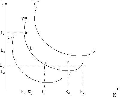
Thus, there is increasing average product and increasing marginal product of labor in this example. Why? One can think of it as follows. When we apply one lonely worker to an entire acre of ripened land, his running around the entire acre trying to harvest it will produce a lower average product than if we had three workers, each working a third of the field by himself. This should already reveal why we would never see a situation of increasing average product. Basically, when we are faced with a situation of a single worker on an acre of land, why should we force him to work on the entire acre and only produce 10 units of output? Average product (and total product) would be higher if instead of forcing that single worker to try to harvest the entire acre, we let him confine himself to a third of that acre, and let the other two-thirds of the plot lie untouched. In this case, the average product of the single worker is as it would have been had there been three harvesters, i.e. 12 units of output. In other words, in situations of rising average and marginal product, total output is increased by discarding two-thirds of the land! Thus, situations of increasing marginal productivity will simply never be seen. Of course, this logic is not unassailable. While the idea may apply naturally to some cases, it can be questioned in cases where division of labor is crucial as, say, we might have in an automobile factory. Suppose that the average productivity of a worker is highest when there are twenty men working on a factory floor, each worker specializing in fitting a special part of the automobile. We cannot subsequently do the same operation we did before. In other words, we cannot remove nineteen men and let 19/20ths of the car remain unbuilt. The only remaining man, whose productivity was highest when he only fitted wheels on axles, will not yield any output if he is permitted to perform only his specialized task bereft of the other nineteen men. Instead of having cars as output in that case, we would have axles-with-wheels. Consequently, we see that in order to produce any cars whatsoever, the lone man must be forced to perform all the tasks, not only the fitting of wheels on axles. If this is true, his productivity by himself, where product is measured in number of cars produced rather than axles-with-wheels, will be lower than if he worked together with his nineteen colleagues. The automobile case shows an example of indivisibility in production, a traditional explanation of increasing marginal productivity (e.g. Edgeworth, 1911; Lerner, 1944). Production is divisible if it "permits any particular method of production, involving certain proportions between factors and products, to be repeated in exactly the same way on larger or on a smaller scale." (Lerner, 1944: p.143). In other words, in a perfectly divisible world, there cannot be changes in method when increasing or decreasing the scale of production. In our automobile example we have indivisibility: when we remove the nineteen men, the remaining man who previously only placed axles on wheels must change his method and do all the tasks in the construction of the automobile. In contrast, our agricultural example was divisible: a laborer working exclusively on his portion of the field will not change his method of harvesting that third of the field when the other laborers on the other the remaining two-thirds of the field are removed. In sum, increasing marginal productivity, especially in cases where specialization is vital, can be ostensibly encountered in the real world where there are indivisibilities in production. Nevertheless, much of the Neoclassical work on the production function omits this. This is, as noted earlier, is often taken axiomatically, but the question of whether one finds it an acceptable assumption is largely an empirical one. The contours along the production "hill" in Figure 2.1 are the isoquants shown in Figure 2.4. A particular isoquant denotes the combinations of factors K and L which produce the same quantity of output. As we are assuming factors K and L are continuously substitutable (on which we will have more to say later), then every point on a particular isoquant represents a particular feasible technique, or factor combination, that can be used to produce a particular level of output. The isoquants play the same topographic role to the production "hill" as indifference curves played in the the "utility hill". As the isoquants ascend to the northeast, the amount of output produced increases, thus Y¢ < Y* < Y¢¢ .
It is an elementary matter to derive the slope of an isoquant. For our two-factor case, we had a production function Y = ¦ (L, K). Now, for the production of a given fixed quantity of output (call it Y*), it follows that Y* = ¦ (L, K). This is the formula for a particular isoquant. Totally differentiating this:
where ¦L = ¶Y/¶L and ¦ K = ¶Y/¶K are the marginal products of labor and capital respectively, evaluated around Y*. Since on any isoquant, output is fixed at Y*, then dY* = 0. This implies that ¦LdL = -¦KdK, or simply:
The term on the left is the negative of the slope of the isoquant corresponding to output level Y*. This is known as the marginal rate of technical substitution (MRTS), i.e. the rate at which capital can be susbstituted for labor while holding output constant along an isoquant. (note that dL/dK by itself is already negative, thus the MRTS will be a positive number). Provided our isoquants are smoothly differentiable, we will be able to define the MRTS at any point in Figure 2.4. Thus, the MRTS depends not only on the level of output (which isoquant we are on), but also the amounts of capital and labor (where on the isoquant we are). The equality of the MRTS with the ratio of marginal products of capital and labor, ¦K/¦L, is a fundamental feature of production theory and helps us capture the concept of diminishing marginal productivity to a factor. In Figure 2.4, on isoquant Y*, as we move from point a to b to c to d, we are moving towards greater employment of K and less employment of L to produce a given level of output Y*, thus we are moving from labor-intensive techniques (i.e. low capital-labor ratios) towards capital-intensive techniques (high capital-labor ratios). Notice also that the isoquant becomes flatter as we move from a to d, thus the marginal rate of technical substitution is higher at a than at d, i.e. MRTSa > MRTSb > MRTSc > MRTSd. Thus, there is diminishing marginal rates of technical substitution as we move from a towards d. Notice that this declining MRTS arises because of the convexity of the isoquants. As we can notice, the declining MRTS effectively can capture something akin to (but not exactly) of the assumption of diminishing marginal productivity to a factor we spoke of earlier. Compare only the points b and c. As MRTSb > MRTSc, then ¦K/¦L|b > ¦K/¦L|c. But point b represents a lower capital-labor ratio than point c, i.e. K/L|b < K/L|c. Thus, we can interpret the declining MRTS as saying that as we move from lower capital-intensity to higher capital intensity (b to c), the marginal product of capital decreases. Reciprocally, as we move from higher labor-intensity to lower labor-intensity (b to c), the marginal product of labor increases. Note that we cannot derive diminishing MRTS from the assumption of diminishing marginal productivity of factors. To see this, consider the production function, Y = ¦ (K, L). The MRTS at any point is ¦ K/¦ L. In order to have diminishing MRTS, then it must be that dMRTS/dK < 0. But as dMRTS/dK = d(¦ K/¦ L)/dK and ¦ K and ¦ L vary with K and L, then we must take total derivatives. Thus:
as dL/dK = -¦ K/¦ L along any isoquant and given that ¦KL = ¦LK by Young's Theorem, then:
or simply:
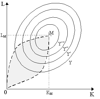
Now, by assumption, ¦ K, ¦ L > 0 and, by diminshing marginal productivity, ¦KK < 0 and ¦LL < 0. This is obviously not sufficient to determine the sign of dMRTS/dK. Specifically, the numerator will only be negative if, in addition, we assume that ¦ LK > 0, and the theory of diminishing marginal productivity implies no such thing. Thus, a diminishing MRTS is, in itself, an separate assumption. We should note, however, that not every point along the isoquant is relevant. The isoquants, after all, are contours of our "production" hill and thus are actually "circular". This is captured in Figure 2.5, where we show the isoquants in their full topographic glory as a horizontal section of the production hill of our earlier Figure 2.1. Notice that the isoquant labels represent increasing output levels, Y < Y¢ < Y¢¢ < Y¢¢¢ , etc. The "top of the hill", the highest output achievable, is represented by point M in the center, achieved by factor combination LM and KM. Notice that if we are the top of the hill, if we increase factor inputs (above KM or LM), output will actually decline.
We have also added dashed "ridge lines" to the topographic map in Figure 2.5. Only those points within the ridge lines, in the lightly shaded region, are of economic relevance. To see why, return to Figure 2.4 and notice that at point a, the isoquant has a vertical slope and a point d, the isoquant has a horizontal slope. Thus, MRTSa = ¦ K/¦ L|a = ¥ and MRTSd = ¦ K/¦ L|d = 0. But our isoquants seem to continue beyond them, yet we assert that points beyond them are economically irrelevant. Why? Consider a factor combination such as at point e in Figure 2.4. Obviously, here, the slope of the isoquant is positive, i.e. dL/dK|e > 0, which implies, in turn, that MRTSe = ¦ K/¦ L < 0, thus the marginal product of one of the factors is negative. This violates the first assumption we made about the production function: namely, that ¦ i > 0 for all i, i.e. increasing the employment of any factor in a production process will always increase output. Thus, we ought to exclude all regions where marginal products are negative. Is this assumption reasonable? Well, notice that at point e, we are employing factors Ke and Le to produce output level Y*. Yet, we could decrease the amount of capital employed to Kd and leave labor at Le in order to achieve a combination at point f. But notice that as point f is above the isoquant Y*, it effectively represents a higher level of output. Thus, if we are at a point such as e, then by reducing factor inputs we can increase output: such factor combinations are therefore not "economical". Consequently we can rule out point e - and, indeed, all factor combinations on the isoquant Y* beyond d in Figure 2.4. Similarly, we exclude points on the isoquant beyond point a for the same reason. The "ridge lines" drawn in Figure 2.5, pass through limiting points of the various isoquants akin to points a and d in Figure 2.4. In other words, at any point on the upper ridge line, MRTS = ¥ for the relevant isoquant, while at any point on the lower ridge line, MRTS = 0 for the relevant isoquant. Thus, we exclude all regions above the upper ridge line and below the lower ridge line as economically irrelevant. Only the lightly shaded area in Figure 2.5 is "relevent". Notice that the ridge lines meet at point M, the "top" of the production "hill". On a more formal note, we should connect the quasi-concavity of the production function to the convexity of the isoquants in general. A function ¦ is quasi-concave if, for any two input bundles x, x¢ Î R+m
In other words, the output produced from a convex combination (i.e. weighted average) of two bundles of inputs is at least as great as the smaller of the two outputs produced using only one or the other input bundles. A special case of quasi-concave function is simply a concave function, namely for any two input bundles x, x¢ Î R+m:
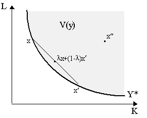
which states that the output produced from a convex combination of inputs is at least as great as the convex combination of the outputs produced by the input bundles independently. The definition of quasi-concavity we used in (A.5) states that V(y) = {x | ¦ (x) ³ y} is convex. In other words, a function is quasi-concave if the upper contour set V(y) is convex. As we see, this "upper contour set" V(y) is merely the isoquant defined by y and the area above that isoquant. This is illustrated in Figure 2.6. Y* is the isoquant of relevance, thus V(Y*), the shaded area, is the upper contour set.
[It is worth pointing out now what the assumption (A.6) on production meant. Effectively, if V(y) has an interior point, then (A.6) intuitively states that for any upper contour set V(y), there is a factor bundle "inside" it (e.g. x¢ ¢ in Figure 2.6). In order to guarantee (A.6), it is common practice in Neo-Walrasian production theory to impose the assumption of free disposibility in production. What this assumption states, effectively, is that if one can produce a particular level of output y with input bundle x, then one can produce an amount of output which is less than y with that same input bundle, x or, equivalently, one can produce the same level of output y with more inputs. The idea is that the producer just costlessly throws away the "extra" that has been produced or, equivalently just throws away some of the extra factors rather than using them. Thus, in Figure 2.6, x¢ ¢ can be used to produce y if the extra amount normally produced by x¢ ¢ is "thrown away" or if the extra factors are just left unused by the producer. The free disposal assumption, then, is meant to guarantee at least the technical possibility of "inefficient" production, and thus interior points to the production set and the input requirement sets. However extensively used in production theory, it might be regarded nonetheless as somewhat stronger assumption than one might wish for and, thus many economists have endeavoured to dispose of it.] It can be easily proven that if a function is quasi-concave in the sense defined earlier, then its upper contour set is necessarily convex. To see this intuitively, let x and x¢ be two points on the same isoquant, thus ¦ (x) = ¦ (x¢ ), as shown in Figure 2.6. Thus, quasi-concavity implies that the output produced by any convex combination of the two points x and x¢ is greater than the output produced by either point individually. In other words, the convex combination of two points on the same isoquant will lie on a higher isoquant. In Figure 6, we see that l x + (1-l )x¢ is indeed within V(y), thus it will lie on a higher isoquant. This implies precisely the convex shape of the isoquant curves which implies, in turn, the convexity of the upper contour set V(y). A final characterization of quasi-concavity makes use of the bordered Hessian matrix. The bordered Hessian matrix of a twice-continuously differentiable function y = ¦ (x1, x2, .., xm) is defined as follows:
where ¦ i is the first partial derivative of the production function with respect to factor xi and ¦ ij are the second derivatives, all evaluated at a particular factor combination x. If the production function is quasi-concave, then we know that the bordered Hessian of that function evaluated at any input bundle x Î R+m will be negative semi-definite, i.e. its principal leading minors will alternate in sign. Specifically:
... etc. Notice that the very first principal minor implies that -¦ 12 £ 0, which is true whether ¦ 1 ³ 0 or ¦ 1 £ 0, so quasi-concavity does not rule out negative marginal products. The second principal minor implies:
as, byYoung's Theorem, ¦ 21 = ¦ 12, this is reducible to:
Now, even if ¦ 1 ³ 0 and ¦ 2 ³ 0 by assumption, there is little implied by this condition. In other words, quasi-concavity of the production function is not sufficient to guarantee diminishing marginal productivities, i.e. ¦ 11 £ 0, ¦ 22 £ 0, etc. In contrast, concavity of the production function is, indeed, enough to yield diminishing marginal productivity. We can verify this by just examining the Hessian for the production function. This is:
where, note, the border is omitted. Concavity implies that the Hessian matrix must be negative semi-definite, by which we mean that the principle leading minors alternate in sign. This implies that:
... etc. Notice that the very first principal leading minor states that ¦ 11 £ 0, i.e. negative marginal productivity for input 1. As we can order inputs anyway we wish, then this effectively generalizes to stating that every factor exhibits diminishing marginal productivity, i.e. ¦ ii < 0 for all i = 1, 2, .., m. Thus, while quasi-concavity cannot guarantee diminishing marginal productivity to factor inputs, concavity does indeed guarantee it. However, we should note that there are special cases when quasi-concavity of the production function guarantees diminishing marginal productivity - namely, under constant returns to scale. We will have more to say on this later.
|
All rights reserved, Gonçalo L. Fonseca
