________________________________________________________
________________________________________________________ (A) Quantity Theory or Liquidity Preference? (A) Quantity Theory or Liquidity Preference? Theoretically speaking, "Monetarism" began with Milton Friedman's article "The Quantity Theory of Money: A restatement" (1956) which was followed up later in Friedman (1968, 1969, 1970, 1971). As Patinkin (1969, 1972) has gone to great pains to note, Friedman's "restatement" has virtually nothing to do with the "Quantity Theory" as understood in its formal sense, but rather it is "a most elegant and sophisticated statement of modern Keynesian monetary theory - misleadingly entitled" (Patinkin, 1969). As David Laidler would later put it, Friedman's paper "could just as well have been called "The Theory of Liquidity Preference - a restatement"" (Laidler, 1982: p.5-6). Friedman protested against this characterization - "[m]y restatement is a restatement of the quantity theory and is not Keynesian in any meaningful sense of the term" (Friedman, 1970). However, Friedman adopts a rather peculiar take on the meaning of both the Quantity Theory of Money and "Keynesianism". For instance, at one point he argues in response to Patinkin:
Thus, in Friedman's conception, the "Quantity Theory" is not necessarily related to long-run money neutrality, although, in his later work, he would actually achieve this result. For Friedman, then, the Quantity Theory is "a term evocative of a general approach rather than a label for a well-defined theory...a theoretical approach that insisted that money does matter." ( Friedman, 1956). Similarly, Friedman perceived the fundamental feature of what he called "Keynesianism" to be its "money-less" quality. This, of course, is not true: in a proper Keynesian model, the real IS side is balanced by a monetary LM side. But, in the 1950s, Keynesians were working almost exclusively with the income-expenditure type of models. These models tended to ignore the monetary side - or at least, to regard money supply fluctutations as being basically adaptive -- and thus effectively inconsequential -- and to underrate the power of monetary policy in favor of fiscal policy. It is this type of 1950s oversimplified "Keynesianism" that Friedman objected to -- and not so much the more carefully constructed IS-LM models (indeed, his 1956 work was one of the great impetuses for the resurrection of "IS-LM" analysis). Thus, while resisting the label, Friedman (e.g. 1968, 1970, 1987) was willing to admit that his 1956 theory was at least a "Keynesian" reformulation of the Quantity Theory and that the differences between himself and the Keynesians were not deep theoretical ones but of a more empirical nature. In this section, we attempt to couch Friedman's propositions within a Keynesian context, rather than a Quantity Theory one, as this was, indeed, the language in which the Monetarist controversy was conducted. However, we should note that other Monetarists, notably Karl Brunner (1970) and Karl Brunner and Allan H. Meltzer (1971, 1972, 1976), have taken Friedman to task for using the IS-LM language and have gone on to build up a rather differently-founded construction in which to ground the Monetarist propositions. Leonall C. Anderson and Keith Carlson (1970) and David Laidler (1973) also provide alternative formulations -- as, of course, do the later New Classicals. (B) Liquidity Preference: Friedman's Money Demand Function Friedman's (1956) theoretical points might have never been necessary had John Hicks carried the conclusions of his famous 1935 paper on money through to his even more famous 1937 one on Keynes. In the former, Hicks explained how the choice of money holdings can be explained in terms of value theory - namely, as a generalized choice problem. In the 1937 paper, he drew the infamous IS-LM model which implied that there were two distinct decisions to be made by agents: a decision on the quantity of savings (IS) and decision of how to allocate those savings among assets in a portfolio (LM). Unfortunately, Hicks failed to realize that his 1935 paper itself implied that these two choices could be married into a single decision. With the exception of Patinkin's masterpiece, Money, Interest and Prices (1956), most economists continued with this dichotomous decision-making implied by simple IS-LM. Milton Friedman's 1956 article attempted to integrate the IS and LM decisions into a single decision - and, in so doing, transformed the liquidity preference theory of money. Succinctly, he proposed that portfolio allocation decisions could have an impact on consumption-savings decisions. To Friedman, choice of money holdings are part of a generalized choice problem - just as Hicks (1935) had originally proposed. In Friedman's words:
Concretely, Milton Friedman proposed a money demand function in the following general form:
where money demand is positively related to permanent income Yp, negatively related to expected interest rates on bonds (rb), the expected rate of return on equity (re) and expected inflation, p e. "Permanent income", roughly the expected average long-run income, can be thought of as Friedman's concept of "lifetime human wealth", as introduced and developed in his own consumption theory (Friedman, 1957). As temporary income shocks do not affect permanent income, then by relating money demand to permanent income, one will not expect money demand to change much over the cycle. The rate of return on bonds and equity represent the opportunity costs of holding money. The rate of return on money is, for Friedman, the "services" provided by holding money (e.g. greater liquidity, etc.) as well as any interest payments on money deposits at banks. Expected inflation, p e, represents the return on holding goods. This last element is the distinctive relationship Friedman adds: namely, that agents hold (durable) goods as assets and will substitute them for money if they expect price inflation (i.e. "capital gains" on holding goods). This is the heart of the "Monetarist" transmission channel. To see the implications of Friedman's theory, recall that in the context of Hicks' (1937) IS-LM, we would have the basic consumption-savings decision in the goods market governed by the flow constraint:
where Yd is aggregate demand and Ys is aggregate supply and dV the change in inventory holdings. In contrast, the asset allocation decision is governed by the following portfolio Walras's Law stock constraint:
where Md/Ms is the stock level of money demand/supply and Bd/Bs the stock level of bond demand/supply (we are treating "bonds" as short-hand for the complex of all alternative interest-bearing financial assets, thus it includes equities). Starting from a position of full equilibrium, an increase in the money supply, Ms, will make the term on the left negative (excess money supply) which necessarily implies that the term on the right will be positive (excess bond demand). As such, the price of bonds will increase and, as we know, the interest rate will fall - bringing the bond market into equilibrium and thus, by Walras' Law, the money market as well. As we see, there are no direct implications of this portfolio adjustment on the goods market. This merely sets the interest rate, which will then affect investment and thus aggregate demand and so, by the multiplier, output. Thus, there is a semi-strict dichotomy between the portfolio adjustment process and the goods market process - portfolio imbalances are only indirectly channeled to the goods market through the resulting equilibrium interest rate. Friedman's (1956) model is broader in that by relating money demand to conditions in the goods market, he therefore has a direct channel by which portfolio imbalances affect aggregate demand and thus output. In other words, Friedman's generalized portfolio constraint looks like the following:
Thus in a money supply expansion, (Ms increase), the term on the left (the money market) becomes negative. However, unlike the naive Keynes-Hicks liquidity preference constraint, this does not necessarily imply excess demand for bonds since the disequilibrium in the money market can be offset by an excess demand for goods. In other words, the excess supply of money can leave the bond market in a market-clearing condition, the goods market alone being out of equilibrium, i.e. we can have Md - Ms < 0, Bd - Bs = 0 and Yd - Ys > 0. By the Keynesian multiplier, then, as there is excess aggregate demand, then output Ys will rise and money demand Md will rise so that the goods market and money market are brought back into equilibrium. Friedman's relationship is entirely sensible and is indeed a useful elaboration upon Keynes's theory of liquidity preference. After all, why should one necessarily assume that excess money holdings should be applied only to the purchase of interest-bearing financial assets such as bonds ? Consumer durables and semi-durables are, after all, stores of wealth too, and yet are "produced goods" at the same time. In other words, excess money holdings can be gotten rid of by purchasing, say, a house or an automobile rather than bonds. Yet, if the portfolio disequilibrium is disposed of in this manner, there will be a direct impact on aggregate demand and thus output. Thus, money supply can affect the economy not only via its indirect interest effect on investment, but also directly through its influence on the purchase of consumer durables as "assets". Notice that so far we have couched everything in IS-LM language and made no use of the Fisherian Quantity Theory. Friedman's transmission mechanism is a definite improvement on the old Keynesian one in that money market disequilibrium can spill over directly into the goods market, but it is still quite "Keynesian". Later, Keynesian economists such as James Tobin (1969, 1982), would move towards an integration of consumption and asset channels which incorporate Friedman's transmission mechanism. As he notes:
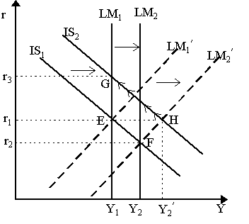
Thus, this transmission channel is, in essence, the full extent of Friedman's 1956 contribution - at least within the confines of an IS-LM representation. However, the Monetarist story does not end there. Friedman's transmission mechanism does not imply that excess money supply always spills over into excess demand for goods; it might still spill over into excess demand for bonds and then we have the standard Keynesian liquidity preference adjustment of money demand and bond demand, with the Friedman transmission channel remaining unused all the while. In order to rule out this last possibility, the bulk of the early Monetarist research program was to prove that the spillover of excess money supply into excess demand for goods was empirically much stronger than the spillover into excess demand for bonds. Some argue that this amounted to showing that, in practice, money demand was insensitive to interest rates - and, indeed, Friedman's 1959 study does move in this direction (although he later retracted this, cf. Friedman, 1966; Friedman and Schwartz, 1982). However, note that such an assumption was not made in his 1956 theoretical work. The difference between the 1956 interest-elastic and the 1959 interest-inelastic versions of the Monetarist transmission mechanism can be illustrated in a simple IS-LM diagram as in Figure 1. Let us take first consider the 1959 version where money demand is assumed to be interest-inelastic and thus the LM curve is assumed to be vertical. Suppose we begin at point E in Figure 1 at the intersection of IS1 and LM1. In this case, an increase in the supply of money will shift the vertical LM curve from LM1 to LM2 and thus achieve a new equilibrium at point F, where we see output has risen from Y1 to Y2 and the rate of interest fallen from r1 to r2. Notice that since we have a vertical LM curve, then aggregate demand movements will not affect output. For instance, if government spending increases so that IS1 shifts out to IS2, as the LM1 curve is unchanged, then we must climb back up the IS2 curve to the new equilibrium G where output remains the same (at Y1) but interest rate has risen from r1 to r3. Thus, in the vertical LM curve characterization of Monetarism, movements in money supply drive movements in output while fluctuations in aggregate demand only affect interest rates and have no effect on output. The policy implications, then, are that only monetary policy is effective, while fiscal policy is completely ineffective.
The vertical LM curve characterization of Monetarism is, as noted earlier, actually inconsistent with Friedman's 1956 article as the latter allowed money demand to be interest-elastic. In other words, the LM curve should properly be considered upward-sloping as LM1¢ in Figure 1. How does the Monetarist transmission mechanism work now? Well, recall that the essence of Friedman's contribution was to claim that excess money supply can feed directly into aggregate demand for goods, thus we must shift both the IS and LM curves in response to a change in money supply. In other words, if we begin at point E in Figure 1 at the intersection of the IS1 and LM1¢ curve, then an increase in the supply of money will shift the LM curve from LM1¢ to LM2¢¢ and shift the IS curve from IS1 to IS2, thus yielding a new equilibrium at the intersection of IS2 and LM2¢ at point H, where we have a higher output level Y2¢ but the same old interest rate r1. Notice the different implications of using the vertical LM and the regular LM characterizations of Monetarism. Firstly, with vertical LM, an increase in money supply necessarily implies a decline in interest rates; with regular LM, an increase in money supply can lead to an increase or decrease or no change in the interest rate; the actual result would depend on the relative size of the shifts on which no a priori assumptions are made. Secondly, with the vertical LM, aggregate demand (and thus fiscal policy) has absolutely no effect on output; in contrast, with the regular LM, aggregate demand (and fiscal policy) can affect output but notice that, relatively speaking, money supply movements nonetheless have a much stronger effect. Although this is an uncommon interpretation (albeit, see Palley, 1993), we believe that the regular LM curve version of the Monetarist transmission mechanism is a much more appropriate and faithful characterization of Friedman's propositions than the vertical LM curve version: it is less outlandish in its assumptions, less stringent in its conclusions, but nonetheless yields effectively the same central message: money supply movements are the strongest (but not the only) drivers of changes in output and monetary policy is considerably more powerful than fiscal policy. The great advantage of the regular LM characterization is that, like Friedman's original propositions, it does not assume that money demand is interest-inelastic and allows the impact of money supply increases on real interest rates to be ambiguous. Nonetheless, many Neo-Keynesians, such as James Tobin (1970) and Franco Modigliani (1977), continued to characterize Friedman's propositions as a vertical LM curve. We believe that a good part of the confusion in the ensuing debate, as captured in Gordon (1974) for instance, rests on the fact that Friedman and his critics could not agree on the characterization of the Monetarist transmission mechanism. The Keynesians insisted that Monetarism implied a vertical LM, while Friedman persistently resisted this. The often harsh and bickering tone of the debate tends reflect precisely this type of misunderstanding, for instance:
(C) Quantity Theory: Friedman Restated This confusion was not assisted by Friedman's recurrent use of the terminology of the Quantity Theory of Money to expound his theory. To clarify why Friedman's theory, at least in the form outlined above, is not the Quantity Theory it might be useful to spend a few moments on this. Irving Fisher's (1911) famous "equation of exchange" states that:
where M is the money supply, V is velocity, P the price level and Y the real output level. The term on the right (PY) is therefore nominal income or nominal output. We can treat this equation not as a tautological identity but actually as a money market equilibrium condition. We can rewrite this as M/P = (1/V)Y, which effectively states that real money supply (M/P) is equal to real money demand (1/V)Y. For the Quantity Theory, the following series of assumptions are then imposed: firstly, nominal money supply M is assumed to be exogenous and thus subject to the full control of the Central Bank; secondly, velocity V is assumed constant; thirdly, the aggregate nominal demand component is assumed to cause changes in nominal income, i.e. causality runs from MV to PY; fourthly, output Y is fixed at the full employment level. The result of these assumptions are far-ranging. Dynamizing our Fisher equation into growth rates:
or:
where gM = (dM/dt)/M, etc. If velocity is assumed to be constant, so gV = 0, and causality is held as in the third assumption, then movements in nominal output (PY) are driven by movements in the supply of money (M). If real output is assumed to be constant at the full employment level, so gY = 0, then gM = gP, money supply growth feeds entirely into price inflation. As real variables (velocity and output) are unchanged by an increase in the money supply, the Quantity Theory thus claims that money is neutral (at least in the long-run). This is the strongest version of the Quantity Theory. We can weaken it by allowing for output growth, gY ¹ 0 and changes in velocity, gV ¹ 0 - with the condition that these growth rates are relatively stable and predictable. In other words, output is assumed to grow at some stable rate of resource growth while velocity is assumed to increase at some relatively stable rate of institutional evolution. In this case, gM - (gY - gv) = gP, so that inflation is driven by the degree to which money supply growth exceeds the term (gY - gv), i.e. output growth minus velocity growth. As the stability assumption implies that the term (gY - gv) is constant, then, once again, excess money supply growth above this determines the inflation rate. Let us analyze each of the assumptions in turn and the degree to which they are contained in Friedman's work. The first assumption of a exogenous and controllable money supply is necessarily problematic due to the nature and definition of money itself. To claim that money is "exogenous", one first of all needs to possess a precise definition of it, but as an aggregate it is subject to different compositions and definitions. Furthermore, much of it is controlled by financial intermediaries, rather than Central Banks. Nevertheless, this is a line of criticism which we shall leave open for the moment, as many Keynesians were willing to entertain the exogeneity assumption. The second assumption of constant or stable velocity is far more controversial. Since V is an unobserved variable, how can one conjecture over its movement? In Friedman (1956, 1970) velocity V is not assumed to be constant. Rather, Friedman explicitly accepts that when the real interest rate rises, velocity rises and thus demand for money (1/V)Y falls. Indeed, his great effort in 1956 was to establish a money demand function which gives choice-theoretic underpinnings to velocity - and interest is one of the primary elements in that function. Most of the Monetarist studies of money demand (except for the aberrant one by Friedman (1959)), do indeed show that money demand is interest-elastic. However, notice that the Monetarist transmission mechanism, in its regular LM characterization, does imply that velocity does not change very much in response to increases in money supply. When we undertook the simultaneous IS and LM shifts in Figure 1, the interest rate remained unchanged and so, in that particular example, velocity would be unchanged. Because the Monetarist transmission mechanism always has these offsetting IS and LM shifts in response to money supply changes, then, as a result, interest rates and thus velocity will tend not to undergo large changes. Thus, while Friedman does not assume that velocity is constant (as many of his critics charged him), his transmission mechanism does seem to be imply nonetheless that velocity will not change much as a result. A relatively stable velocity is a consequence not an assumption of Friedman's mechanism. We can restate all this in Fisherian terms. The implication of the Monetarist transmission mechanism is that if M rises, then as V will not change by much, then PY will have to rise to the full extent to which M has risen. In constrast, in simple Keynesian IS-LM models, increases in money supply (shift in LM alone) do not have as large an effect on nominal output. Translated into Fisherian terms, in the Keynesian model, part of the increase in M is absorbed by a fall in V (due to falling interest rates), so that nominal income PY does not need to rise as much. Much of the dispute between Monetarists and Keynesians, then, is over the extent to which money supply increases make their impact felt on nominal output. Monetarists argue that the full impact is felt, Keynesians argue that velocity absorbs a good part of the impact -- and thus that the effect on nominal output is much smaller. The next assumption necessary for the Quantity Theory is that output is constant or growing at some constant rate. It is extremely important to note that Friedman (1956) does not make this assumption. Friedman does not try to pin down Y or gY independently. Money supply, Friedman asserts, drives nominal income, PY, and he does not specify whether this is a rise in prices or a rise in output or a bit of both. There is, as he put it, a "missing equation" which would specify which proportion of the change in PY is a rise in P and which proportion is a rise in Y. However, the proposition of long-run "neutrality", i.e. that money supply only affects prices in the longer-run, is one of the central tenets of the Quantity Theory of Money. Thus Friedman's refusal to assume that output is constant or growing at a constant rate is one of the major pieces of evidence that his 1956 theory is not a restatement of the Quantity Theory, understood in the proper sense. It is only in later years, notably after Friedman (1968), that Monetarists managed to pin down output with a "natural rate hypothesis" and thus claim that, at least in the long run, real output does not change and prices do all the adjusting. Thus, it is only after 1968 that the Monetarists can claim to have something akin to a "Quantity Theory". But at least in the early debates surrounding the Monetarist transmission mechanism, this was not a point of contention. The final assumption of the direction of money-income causality was a central feature in Friedman's theory and became the curious point of dispute between Keynesians and Monetarists. Keynesians accept that increases in money supply affect nominal income - after all, a shifting LM curve does affect output in Keynesian IS-LM models. It was Friedman's assertion that this was the strongest and most common, if not the only, source of output fluctuations that caused the furor. We turn to this "money-income causality" debate next.
|
All rights reserved, Gonçalo L. Fonseca