Although Michal Kalecki had been independently working on business cycle theory before Keynes wrote his General Theory, Kalecki's various contributions have since been incorporated into the corpus of "Keynesian" literature on macrodynamics. His early 1935 model used a linear difference-differential equation mix to yield cycles and his 1954 work used linear systems with exogenous shocks, but his work in 1937 and 1939 used effectively a non-linear system to obtain endogenous cycles. Kalecki's "distribution" cycle related dynamics and income distribution in perhaps the first mathematically sophisticated treatment of cyclical phenomena in economics. His instrumental relationship was to posit a lag between the investment decision and installation of investment goods. This concept was actually used by Harrod to explain the lagged structure of the accelerator: production takes time, and the "interval that elapses between placing an order for, or beginning to undertake the construction of, capital goods and their use in the productive process can hardly be neglected" (Harrod, 1936: p.88). However, for Kalecki, the decision to invest is dominated not by an accelerator mechanism but rather by a "profit mechanism". Entrepreneurs make profits and these profits are then invested - and thus the greater the profit reaped, the greater the amount of investment will be. As profits are the return to capital, then the distribution of income between capital and labor becomes one of the central factors for Kalecki's system - marrying, therefore, the spirit of Marx to that of Keynes. The following formalization of the Kalecki model in continuous time is due to R.G.D. Allen (1963) and is found in Gandolfo (1971) and Gabisch and Lorenz (1987). Let D(t) be the investment decision and let I(t) be the actual installation of investment equipment. Then, let q be the fixed time interval required between investment decision and installation, so:
or:
i.e. any actual investment at time t would have been derived from a decision to invest at time t-q . Between the time of decision and installation of investment capital, investment goods will be produced. The value of undelivered investment goods at any time t is the amount of investment decisions which were made within the fixed period q before it, i.e. decisions made between t-q and t. As we are in continuous time, the value of undelivered investment goods equals:
As q is a number, then the average value of investment goods per unit of time is A(t) = W(t)/q or:
or, as I(t+q ) = D(t):
But I(t +q ) = dK(t +q )/dt , so solving:
thus, investment per time period is equal to the average change in capital. This A(t), then, is the investment spending at time t. Decision to invest is based positively on profits P(t) and negatively on capital K(t). Kalecki argued that income is decomposed into profit income (to capitalists) and wage income (to workers) and, for simplicity, that workers consumed all their income and, correspondingly, that capitalists saved all of theirs. Thus, profits P(t) = sY(t) where s can be interpreted in the Marxian vein as the share of income going to capitalists or in the Keynesian vein as s = (1-c), the marginal propensity to save. The relationship between profits and investment decision can be argued on various grounds, but Joan Robinson's succinct summary of the Kaleckian argument is that capitalists invest their profits because it "offers more favorable odds in the gamble and because it makes finance more readily available" (Robinson, 1962: p.38). Thus, Kalecki's investment decision function would look something like:
where F (., .) is non-linear in Kalecki (1937) but linear in Kalecki (1935) as follows:
where s, d > 0. Goods market equilibrium requires that Y(t) = C(t) + A(t), where consumption C(t) = cY(t) = (1-s)Y(t) and investment A(t) is as derived before so that:
thus, plugging this into the 1935 linear D(t), the decision to invest can be rewritten as:
or, reorganizing:
But recall, from before, that D(t) = I(t+q ) = dK(t+q )/dt. Thus:
or, lagging everything back q periods:
which is the mixed difference-differential equation which summarizes the Kaleckian system. Solving this system would take us a bit far afield, therefore we prefer to refer to Allen (1963) for details. The sum argument is that this is akin, in result, to the multiplier accelerator model as only very specific values of the parameters d and a would we obtain constant cyclical fluctuations. To get out of this structurally unstable requirement, Kalecki (1935, 1954) appealed to continual exogenous stochastic shocks in the manner of Frisch-Slutsky to drive a damped oscillating system into continuous cycles. Kalecki (1937, 1939), however, appealed to non-linearity of the function D(t) = F [sY(t), K(t)] and we shall follow this heuristically. We can relate D(t) to Y(t) in non-linear fashion similar to Kaldor's (1940) investment function - and the same underlying economic argument can be made, i.e. that at extreme values of Y, sensitivity of investment to income declines due either to excess capacity at low income or rising supply price/full employment constraints at high output. This is shown in the Figure 1 and is similar in form to the accelerator of our earlier models - but not the same (recall the underlying "profit mechanism" of Kalecki's system). We also saw that, Y(t) = C(t) + A(t) and from this we obtained Y(t) = (1/sq )[K(t+q ) - K(t)] which we can summarize heuristically as Y(t) = ¦ (dK(t)/dt). We also know that dK(t)/dt = D(t-q ) or, normalizing q = 1 and inputing that in:
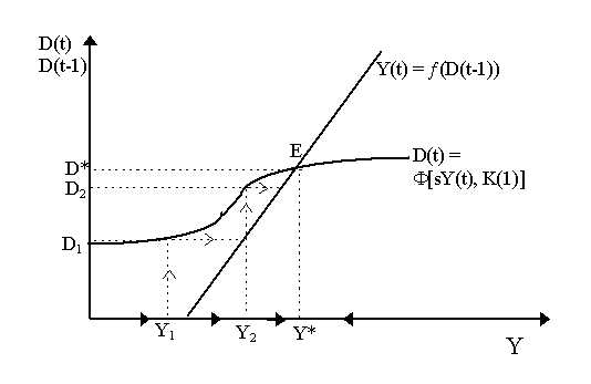
so that output in period t is some function (positive) of past investment decisions. This is analogous to the "multiplier" relationship in more strictly Keynesian models. This is assumed a positive linear relationship and is drawn in Figure 1. The dynamics of Kalecki's system work essentially as follows. Given an initial stock of capital, K1, then starting from an initial output level Y1, we obtain, as a result, a set of profits P1 = sY1 which feed into the decision function at time t = 1, D(t) = F [sY(t), K(1)] to yield D1. In the next period, as Y(t) = ¦ (D(t-1)), then Y increases from Y1 to Y2. If we temporarily (but erroneously) assume that capital remains constant at K(1), our function D(t) remains unchanged and thus the rise in Y to Y2 will subsequently lead to an increase in investment plans from D1 to D2 -which will in turn increase output toY3 and so on until we reach an equilibrium such as point E at (Y*, D*)
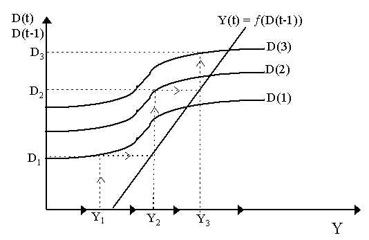
However, capital is not constant and thus it is misleading to keep the D(t) curve constant. In effect, as Y1 is very low, then capital should decrease as there will be insufficient investment to cover replacement. The fall in K from K(1) to K(2) will shift the D(t) curve up from D(t) = F [sY(t), K(1)] to D(t) = F [sY(t), K(2)] and thus we bounce off this second curve to obtain D2 from Y2 and not off the first curve as is obvious in Figure 2. If Y3 obtained from D2 is still sufficiently low, capital should decrease again to K(3) and thus the D(t) curve should shift up. This is obvious from the diagram below where D(1), D(2) and D(3) denote the curves D(t) = F [sY(t), K(t)] where K(t) = K(1), K(2), K(3) respectively.
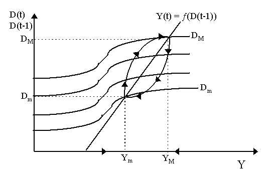
It may seem we no longer have stability in this case, but this is not exactly true. The decisions to invest will eventually be implemented and capital will begin to be added which will slow down the ascendancy of the D(t) curves until they are stopped altogether and begin to fall in the other direction. Recall that when capital increases, D(t) falls, thus when capital implementation is greater than depreciation, the decision will be to reduce capital and thus D and Y begin climbing down, as shown in Figure 3. However, cutbacks in investment decisions, even disinvestment, will not last forever either: as the old capital projects are implemented, capital accumulation still exceeds depreciation and firms will cut back decisions; but as there are fewer and fewer past projects to implement, capital accumulation slows down until it is no longer sufficient to cover depreciation, and thus total capital stock begins to fall - thus D(t) begins to rise again. The process has thus an endogenous ceiling and floor and cyclical behavior between them.
A heuristic portrait of the Kaleckian cycle is shown in the Figure 3 where we climb up the left side up to DM (the maximum decision curve) and climb down the right side to Dm (the minimum curve) which define the limits of the process. They also define the highest (YM) and lowest (Ym) values of output and output will cycle between these values. Of course, complete cycles should only emerge in particular parameter ranges, for it it not entirely inconceivable that stability can result if some adjustments are faster than other.
|
All rights reserved, Gonçalo L. Fonseca