One may argue that the components of Hicks's (1950) growth cycle model, ceilings, floors and an exogenous rate of growth of autonomous investment (equal to the rate of growth of factor supplies) is unsatisfactory. These exogenous factors are, indeed, quite arbitrary and, as their values can be anywhere, there does not seem to essential cycles. A way to circumvent this is to appeal to theories which obtain growth and cycles endogenously. Non-linear cycle models were developed precisely for this purpose. However, the simplest alternative procedure to obtain growth and cycles endogenously would be to modify the Hicks model with Duesenberry "ratchet" effects on consumption and/or Smithies "ratchet" effects on investment - more complicated non-linear models being left for later. James Duesenberry (1949) proposes a consumption function which accounts for some adjustments for "habits" or "standards of living". Conventionally, if income falls, then consumption should fall proportionally with the marginal propensity to consume. Duesenberry rejected this: once consumption habits are acquired, it is hard to get rid of them. Thus, income shocks should have slightly different effects on consumption. Certain consumption habits are formed at high income levels which are not completely abandoned when income falls. This effect is captured in the following consumption function:
where Yt-1m is the maximum level of income before time period t. Thus, consumption habits acquired when income was at its highest influence present consumption decisions. Unlike Duesenberry, Arthur Smithies's (1957) "ratchet" effects are actually applied to the investment function rather than to the consumption function and they also end up yielding cycles around a growth trend. However, we shall stick mainly to the Duesenberry consumption function and omit the Smithies ratchet - thus we presume the investment function has the same presumed to have the same properties as before (now without depreciation) so:
thus, for goods market equilibrium:
or:
which is our old Hicksian second order linear difference equation - only now with the term c2Yt-1m involved among its autonomous components. Without looking too carefully, one might suspect that the only effect would be then that the particular numerical value of the equilibrium level of output would be different. But in fact, the effect of adding a "ratchet" to consumption is more substantial. Namely, we have changing parameters and changing steady-state equilibria. This is easy to see. Suppose that Yt-1m is far in the past - call this case 1. In this case, then, the particular solution (equilibrium) to the difference equation is:
where, assuming that c1 = c (our old mpc), our characteristic equation is now:
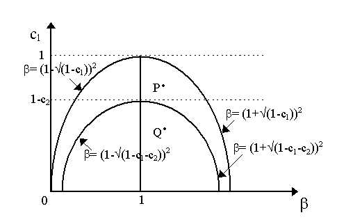
then we can just draw this as in the old Hicksian (b , c1) space as in Figure 1 below. The only difference is that our curves are now b = (1 - Ö (1-c1))2 and b = (1 + Ö (1-c1))2 where again monotonicity is defined when b is above this and oscillation when it is below and the border between stable and unstable dynamics remains b = 1. Thus, nothing substantial changes except the numerical value of the equilibrium. But now suppose that an economy is growing. Then, in this case, call it case 2, Yt-1m = Yt-1, i.e. last period's output is the maximum output. Thus, for case 2, the difference equation becomes:
so that the particular solution (equilibrium) is:
which is different from that of case 1 as now c2 enters in the denominator as part of the multiplier. Similarly, under case 2, the characteristic equation becomes:
which is very different from case 1. It is easy to see that the curves for the parameter constellations in (b , c1) space are now:
and:
which are different from case 1. Thus, the boundaries we had before now shift "in" as shown in Figure 1. When b = 1, now, c1 = 1 - c2 and not 1.
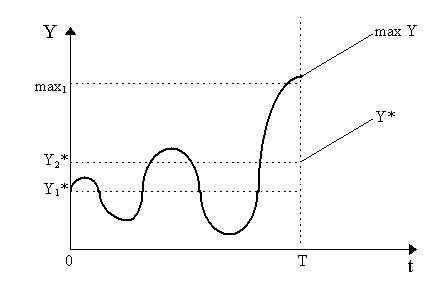
What are the implications of this? Well, quite simply, the properties of the parameters change during the cycle - thus one may consider it somewhat "non-linear". Let us consider two cases: that of points P and Q in the figure above. For the sake of simplicity, we shall assume henceforth that the exogenous rate of growth for autonomous investment is zero, i.e. g = 0 so that I0egt = I0. Thus, our equilibria Y* are constant. Suppose we have specific values of b and c1 (assumed constant) at point P. Then we alternate between explosive oscillations to explosive monotonic dynamics. This is not altogether very interesting. The situation is illustrated in Figure 2. Suppose we begin at a time when Yt-1m is max1. Then, from t = 0 to t = T, the maximum is long in the past (max1) and our equilibrium is Y1*. Under this, then, we have case 1 and thus explosive oscillations. So, as we begin from time t = 0, Y has explosive oscillations.
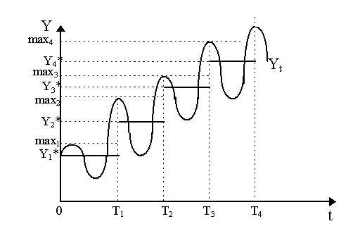
However, eventually, as the swings of Y are growing, we shall get a value of Y which is greater than max1. In our case, Y achieves and surpasses max1 at t = T (or rather, just before that) in Figure 2. As a result, case 2 comes into effect. Now, we have two things: firstly, a new, higher equilibrium (Y2*) will result and a new higher maximum will be established corresponding to the Y achieved at t = T. However, as we now have explosive monotonic dynamics, then Y will not move down towards the new equilibrium Y2*. Instead, it will continue to explode upwards. But as it explodes, it will create a new higher maximum Y and thus a new higher equilibrium Y* after T. But the explosive monotonicity maintains itself so again, the maximum continues to grow and Y* continues to grow. This is shown by the two lines Y* and max Y after t = T in the figure above. The case of P, illustrated in Figure 2, is not that interesting for we move from oscillations into monotonic explosions which eliminates the cycle. However, suppose we were with a parameter constellation such as Q in Figure 1. Then, both before and after the parameter changes, we would still have explosive oscillations. This case is illustrated in Figure 3 below. We begin, again, at t = 0 with a maximum Y (= max1) and equilibrium Y1*. We have explosive oscillations and these continue until we hit t = T1. Then, our upward swing of Y moves above max1 all the way to max2. This becomes the new maximum and, as a result, the new equilibrium is Y2*. However, given that we still have explosive oscillations, output falls after t = T1 and, indeed, falls below the new equilibrium. But, as we have explosive oscillations, then sometime in the next upswing, at t = T2, Y rises above max2 all the way to max3. This creates a new maximum (max3) and a new, higher equilibrium Y3*. Again, because we have oscillations, then from t = T2 to t = T3, the rest of the cycle works itself through normally until, of course, during the upswing, at t = T3, again we surpass the old maximum to obtain a new maximum (max4) and a new higher equilibrium, Y4*.
We can see now what is happening in Figure 3. The equilibrium Y* is rising stepwise and oscillations are happening around this equilibrium. Obviously, then, we have Harrod's grail of growth with cycles: Y* increases while actual Y = Yt is moving in cycles along this increasing equilibrium. This is the result of parameter constellations such as Q when you add Duesenberry (1949) "ratchet" effects on consumption on the simple Hicksian multiplier-accelerator model: cyclical growth without once the need for the Hicksian paraphenelia of exogenous growth rates, ceilings or floors. If we had assumed a positive exogenous growth rate (g > 0), then the equilibrium Y* would be steeper (i.e. the steps would have been greater) - perhaps to a point where the downswing would result in only slightly or even no negative growth of output. Amplitudes of the cycles, of course, should not be assumed constant but probably increasing over time.
|
All rights reserved, Gonçalo L. Fonseca