John Hicks (1950) is credited for trying to reveal proper macroeconomic cycles in a linear multiplier accelerator model by essentially aiming for unstable oscillations and adding floors and ceilings to constrain them. However, Hicks proposed a slightly different model. Instead of having the accelerator related to past consumption changes, he had it related to past output changes, in short he argued that:
where, note, we are pulling two periods back. He keeps the same simple Robertsonian consumption function we had for the Samuelson case:
thus, in goods market equilibrium:
or simply:
again, we can rewrite the system as a second order linear difference equation:
The particular solution (equilibrium) is:
or:
which is identical to Samuelson's (1939). However, the characteristic equation is:
which is different from Samuelson's. The eigenvalues are then determined as:
where, again, we can derive different parameter regimes for b and c, as illustrated in Figure 1. The discriminant now is D = (c+b )2 - 4b . So, for regular dynamics, D > 0, then (c+b )2 > 4b or c+b > 2Ö b so, rearranging:
which can yield two results
or:
So, rewriting the first, 1 - Ö b > Ö (1-c) or -Ö b > Ö (1-c) - 1 thus multiplying through by -1 and taking the square:
so the condition is fulfilled here. Doing the same with the second, we obtain:
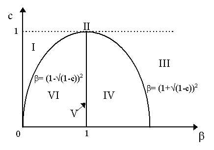
In Figure 1, we have drawn the two curves, b = (1-Ö (1-c))2 and b = (1+Ö (1-c))2 which meet at point II. Note that when c = 1, then b = 1, thus the maximum c is 1 and that maximum will be at b = 1. Note also that as regular monotonic dynamics require that b be greater than both curves so, above the curves (areas I, II and III), we obtain regular, monotonic dynamics. What about the stability or instability of the equilibrium? Well, it can be easily shown that if:
then we have stability (area I) and if:
then we have instability (area III) whereas if b = 1 we have constancy (point II). What about complex roots (when D < 0)? Well, following our old modulus argument where now a = (c+b )/2 and b = (-D)/2, then:
or:
as Ö (a2 + b2) = Ö 1 = 1 = a2 + b2, then we get unstable oscillations if b > 1 (area IV) and stable oscillations if b < 1 (area VI). Figure 1 summarizes the Hicks (1950) parameter regimes.
Again, we have six areas of parameter constellations for different dynamics:
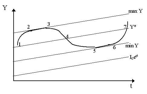
Again like the Samuelson case, it is only when parameter values (b , c) fall in region V that we obtain regular cycles. Note, however, that to obtain V, all we have to do is obtain the value b = 1 for any c will be compatible with that. In Samuelson's multiplier-accelerator model, we were forced to obtain precise values of both c and b to get case V of constant oscillations. It seems that Hicks' multiplier-accelerator model remains equally insufficient as a theory of the cycle. Constant cycles can be obtained, but they will not be structurally stable (as any slight movement of b above or below 1 will lead to explosion or stability). However, Hicks (1950) proposed that we add several things to our this basic MA model: namely, ceilings, floors and a exogenous constant growth rate of autonomous investment. This enables us to obtain growth with cycles. The logic is simple. Investment, as we know, is composed of two parts: autonomous investment, I0 and induced investment (induced by the accelerator, b (Yt-1 - Yt-2)). Now, Hicks proposed that for a growing economy, "autonomous investment itself will have to increase at a constant rate of growth" (Hicks, 1950: 59). Let us propose this constant growth rate to be g so that autonomous investment at any time period t is I0egt. Also, investment adds to the stock of capital, thus the greater investment is, the greater the stock of capital becomes. However, capital depreciates. Thus, some amount of investment will not result in a net increase in capital stock but rather only serve to replace existing, depreciating capital stock. Now, suppose we are in the downswing or trough of the cycle such that induced investment is zero (as output growth is negative or constant). In this case, all investment is autonomous (I0egt). This is shown in the figure below. Net investment becomes in this case:
where d is depreciation (level, not rate, and assumed constant). Now, for the capital stock not to start decreasing (and thus the multiplier not to amplify negative effects), then It ³ 0. Thus, we can assume that this places a "floor" on the system. Actual investment cannot fall below d . But as there is an exogenous rate of growth of autonomous investment, then that floor is not constant. Simply, as I0egt is growing over time (and d is not), then It at its minimum must also be growing at rate g. This is shown in Figure 2 as min Y. (note: it actually should not have exactly the same slope as the autonomous investment function because as d is constant, then min Y should be steeper, but that only makes a slight difference so we draw them as the same, cf.Hicks, 1950: p.102). In short:
Hicks then also proposes a ceiling. Output cannot grow indefinitely due to restrictions in factor supplies. Greater output may be demanded, but if one is at full employment, the only possible result is that the prices of these factors will rise - more supply will not be forthcoming. Assuming factor supplies also grow at the exogenous rate g, then the maximum output level also grows at rate g. This ceiling is shown in Figure 2 as the line max Y. What Hicks (1950: Ch. VIII) proposes is then quite simple to explain. Namely, suppose b and c assume values such that we obtain explosive oscillations (case VI). With floor and ceiling imposed, both growing at rate g, then oscillations in output are confined within ranges of values between max Y and min Y - both of which are growing at the exogenous rate of g. Similarly, the equilibrium level of output is also growing at rate g. This is easy to determine since equilibrium Y is defined as:
thus equilibrium output also grows at rate g (as shown in the Figure 2).
Due to the presumption of depreciation then the investment function becomes:
Now, suppose we begin at point 1 in Figure 2. Obviously, we are in an upswing therefore output is growing so that the accelerator will be working and thus induced investment exists. Thus, the function which applies is I0egt + b (Yt-1 - Yt-2). Obviously, then, investment is growing at a rate greater than g. Thus, from point 1, output grows faster than g. However, soon we hit the ceiling (point 2). As factor supplies cannot grow faster than g, then output is forced to grow only at rate g. Thus, as time progreses, we move from 2 to 3, i.e. output moves along the ceiling at rate g. Now, as output is still growing (at rate g, though), then the accelerator will still be working. However, net investment will be less than that which took us to the ceiling. Thus, as investment becomes less, then the maximal level of output is not sustainable by that level of investment (via the multiplier). Thus, output will have to move back towards the equilibrium. Thus, from point 3 we move towards point 4. But between 3 and 4, output is falling thus, b (Yt-1 - Yt-2) becomes negative. This will result in negative induced investment. Thus, again by the multiplier, output growth falls and falls at a fast rate. Eventually, of course, induced investment falls below depreciation, i.e. b (Yt-1 - Yt-2) < d , in which case, as per our investment function, the multiplier is eliminated and the only level of net investment will be I0egt - d . Thus, the multiplier is knocked out during the downswing. However, this level of investment cannot sustain high level of output, so output will continue to fall. When the falling Y hits the equilibrium Y*, the fall will not stop - as that equilibrium requires a positive level of induced investment. During the downswing, that value will be zero or negative. Thus, it moves beyond point 4 and towards point 5. At point 5, however, output hits the floor min Y. This, of course, is entirely sustainable by I0egt - d which thus implies that output will stop falling. However, given that autonomous investment is rising at its constant rate, then the multiplier will be brought back into positive effect so that Y grows now along the floor at rate g (e.g. from 5 to 6). But as output grows along the floor, then b (Yt-1 - Yt-2) becomes positive and some induced investment will begin to arise. Eventually, around point 6, I0egt + b (Yt-1 - Yt-2) will become greater than I0egt - d so that the first part of the investment function kicks in. Thus, output will soon begin growing faster than the rate g and we move away from the floor and back up away from point 6. Eventually, of course, we reach the equilibrium level of output, Y*, again - this time at point 7. However, the propulsion provided by the accelarator from the previous rapid growth from 6 to 7 will carry Y above Y* and back towards the ceiling. We have outlined the simplest growth cycle model of Hicks (1950). There is growth at all times due to the exogenous growth of autonomous investment. But the rate g is necessary not only for cycles with growth but also for the existence of cycles themselves. If we eliminated g, then Y* and min Y would be flat and the cycle would end. Simply, as Y would hit min Y, then it would not rise again as induced investment would not kick back in. Thus, only three-quarters of the cycle could be explained.
|
All rights reserved, Gonçalo L. Fonseca