________________________________________________________
________________________________________________________ Contents (A) Factor Payments and the Concept of Rent (A) Factor Payments and the Concept of Rent The first thing to remember is this: in Neoclassical theory, factor prices and quantities employed are determined simultaneously by the supply and demand for factors. Period. If any of the ensuing discussion seems confusing, one can regain one's bearing by reminding one's self of this. This is the thread out of the labyrinth which follows. The second thing to remember is this: in all that follows, there are no produced factors of production, i.e. there is no capital. More precisely, for the rest of this discussion, the word "capital" is used in the same sense as "land", i.e. capital is assumed to be an endowed factor of production (which effectively contradicts the definition of capital! -- but more on that later).. For an analysis of the theory of distribution with capital properly speaking, turn to our discussion of capital theory. The reason for these initial warning is that the Neoclassical theory of distribution -- what has become known as the "Marginal Productivity Theory of Distribution -- has been a subject of much debate and confusion since it was formulated in the 1890s. We shall survey this debate here. Before proceeding, we ought to be clear about a few terms. By "distribution" we mean the relative income received by the owners of factors of production. If L units of labor are employed in the economy, each unit being paid a wage w, then the income of laborers (the owners of labor) is wL. If K units of (fixed, endowed) capital are employed and paid a return r, then the income of capitalists (the owners of capital) is rK. If we denote by Y the economy-wide level of output, then the income share of labor can be expressed as wL/Y and the income share of capital is rK/Y. Consequently, the relative income shares of the capital and labor can be expressed as a ratio wL/rK. The distribution of income is about how total output in the economy Y, is divided up among people. Edgeworth called it "the species of exchange by which produce is divided between the parties who have contributed to its production " (Edgeworth, 1904). The laborers get wL, the capitalists get rK and, possibly, there might be some residual amount. This residual amount, the amount of income/output produced which is not paid back to the owners of capital and labor for factor services, is R = Y - rK - wL. The residual is usually paid out to a the class of people known as entrepreneurs. It is important not to confuse this "residual" with the "surplus". The "surplus" is defined as the amount of output that is not paid out to factors in reward for "factor services." So, if we define r and w as the rate of return and wage in "reward" for factor services, the surplus is defined as S = Y - rK - wL. This seems mathematically similar to the entrepreneurial residual, but it is, in fact, quite different. Explicit in the definition of the surplus is the assumption that r and w are what is called "economic earnings" alone. In contrast, the r and w in the definition of the entrepreneurial residual include both economic earnings and "rental earnings". So, if we define re and we as the economic earnings of capital and labor and rr and wr as their "rental" earnings, then the surplus is: S = reK + weL while the entrepreneurial residual is: R = (re+rr)K + (we + wr)L So, implicitly, while the residual accrues to the entrepreneur alone, the "surplus" includes amounts that accrue to labor and capital in the form of rental earnings. This may all seem a bit obscure and so we need to define things a bit better. Just how do we distinguish payments for factor services from payments derived from the surplus, i.e. between economic earnings and rental earnings? The difference differs in meaning between Classical and Neoclassical economists. However, in general, we can define them as follows:
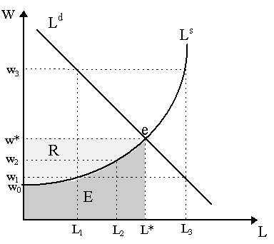
Turning to economic earnings, what does "necessary and sufficient to employ a factor" mean? For the Classical Ricardian school, the economic earnings of a factor are merely the payments necessary to maintain the factor "intact". Thus, for laborers, economic earnings are wages required to keep the laborer alive and well, i.e. "subsistence" wages. (for capital, the story is more complicated; see our discussion of Classical capital theory). Although some Neoclassicals have agreed to this Classical definition, most have taken on the Austrian definition of economic earnings in terms of opportunity costs. If a producer wishes to secure the employment of a particular factor, it has to pay that factor at least what it might receive in alternative employments. This is the opportunity cost of the factor. So, if a factor is paid $7 an hour by a particular producer and could find alternative employment only for $5 an hour, then the factor's opportunity cost (and thus its economic earnings) are $5 and its surplus earnings are $2. We can fix our ideas better by examining the factor market equilibrium for a particular factor. An example for the labor market is shown in Figure 1. The Ld curve is the economy-wide demand for labor by firms, Ls is the economy-wide supply of labor by households. The demand for labor is downward sloping with respect to the wage for reasons that have already been extensively analyzed in the Neoclassical theory of production: specifically, as the wage increases (holding all other factor prices constant), firms will choose techniques of production that substitute away from labor and towards other factors. We know, from profit-maximization, that they will choose to employ labor until the marginal value product is equal to the wage. Thus, heuristically, the labor demand curve Ld can be seen as the economy-wide marginal value product of labor curve (if we can define such a thing as an economy-wide MVP!). The labor supply curve is upward sloping because of labor-leisure choice issues: the greater the wage, the greater the opportunity cost of leisure, and thus the more households substitute away from leisure and towards labor.
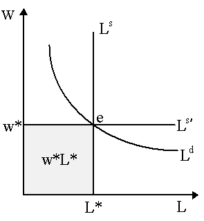
Factor market equilibrium is established where the economy-wide demand for labor Ld is equal to the economy-wide supply of labor (Ls). In Figure 1, this will be at w*, where Ld = Ls. Notice that at a lower wage, e.g. w1, there is an excess demand for labor as Ld = L3 > L1 = Ls. At a higher wage, e.g. w3, we have excess supply of labor as Ld = L1 < L3 = Ls. The wage w* in Figure 1 is the equilibrium wage. Equilibrium quantity is L*, thus economy-wide labor earnings are, in equilibrium, w*L*, the area of the box formed by 0L*ew* in Figure 1. Economic earnings and rental earnings are noted in Figure 1 by the areas E (for economic earnings) and R (for rental earnings). The reasoning for labelling the R and E areas in this manner can be readily understood. When we are at the factor market equilibrium (w*, L*), every worker is individually paid the equilibrium wage, w*. However, it may be that some of these workers might have been willing to work at a lower wage. They nonetheless receive w*. For instance, notice in Figure 1 that at wage w1, the amount of labor supplied is L1. Thus, the "economic earnings" of the first L1 workers, the payment that would have been sufficient to command their labor, is not more than w1. However, in equilibrium, these same set of workers, L1, are paid the equilibrium wage w*, which is considerably higher than w1. This principle applies to all the "intramarginal" workers supplied between zero and L*. Thus, the area below the labor supply curve reflects economic earnings, while the area above the labor supply curve reflects, as we shall see, rental earnings. We spoke earlier that economic earnings are payments required to command labor, which, we noted, in the Austrian sense, are conceived as opportunity cost payments. Opportunity cost is captured by the shape of the labor supply curve. In this simplified scenario, we can conceive of the "alternative" employment of the laborers to be "leisure". Thus, the greater the "rewards" of leisure, the lower will be the labor supply at any wage rate (i.e. Ls shifts left) and thus the greater the wage required to command any laborer and thus the higher the economic earnings of any employed laborer. Note the implications of the two extreme scenarios, both depicted in Figure 2. Suppose leisure is so disliked that, in fact, workers do not consider it a gainful alternative to employment. In this case, the labor supply curve is vertical as shown by Ls in Figure 2. In other words, any wage rate will call forth the entire labor force. Now, equilibrium will still be where the labor demand and vertical labor supply curve meet at e, thus we still have a strictly positive equilibrium wage, w* > 0 and strictly positive labor earnings (the area of the box, w*L*). However, notice that now that all earnings of labor, w*L*, are rental earnings and economic earnings are nil. Conversely, suppose labor supply is supplied with infinite elasticity, i.e. we have a horizontal labor supply curve such as Ls¢ in Figure 2. In this case, an infinite amount of labor is supplied when the wage is greater than w* and no labor is supplied when the wage is below w*. Labor earnings are still defined at equilibrium e as the area of the box w*L*. However, note that now equilibrium labor income w*L* will be entirely composed of economic earnings and no rental earnings are received.
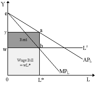
The reasoning for these two extreme cases is readily apparent. When the labor supply is inelastic (vertical Ls), i.e. when there is no alternative employment, then any earnings made by labor must necessarily arise because firms are fighting over a limited supply of them. In other words, firms are bidding up their wages "artificially" above what is necessary to get them to work. The supply of workers will be L* regardless of what the wage offered is. As such, workers are experiencing a windfall gain in this case: they would be willing to work for less, much less (indeed, near zero), but competition among firms has bid their wages up regardless. In contrast, when the labor supply is perfectly elastic (horizontal Ls¢), then there are no "intramarginal" workers. In other words, at least w* is necessary to call forth any labor and, furthermore, w* calls forth an infinite amount of labor. Labor supply is not finite at w*. This implies that, as long as firms pay at least w*, they do not need to "fight" each other over a limited supply of workers. As there is no "bidding war" ensuing from limited labor supply, firms will have no incentive to pay workers above their minimal opportunity cost wage, w*. These examples permit us to better define the meaning of rental earnings of a factor as that portion of earnings that arise purely out of the fact that the factor is in fixed supply. This concept of rent, or differential rent or Ricardian rent as it has been variously called, was introduced simultaneously but independently by T.R. Malthus (1815), Robert Torrens (1815), Edward West (1815) and David Ricardo (1815), and became one of cornerstones of the Classical Ricardian theory of distribution. Classical theory generally did not assume that factors were fixed in supply: in other words, they assumed that capital and labor could be "produced". In terms of Figure 2, they believed the labor supply curve was horizontal so that all payments to labor were economic earnings. However, following David Ricardo (1815, 1817) they recognized that land was fixed in supply and thus that land made rental earnings. Figure 3 illustrates the Classical Ricardian theory of rent. Here we are assuming only two factors of production: labor (L) and land (T), where the labor is completely variable but land is in fixed supply. The production function is thus Y = ¦ (L, T0), where T0 is the fixed total supply of land. In contrast labor is supplied with infinite elasticity (a typical Classical assumption). This is captured in Figure 3 by the infinitely-elastic labor supply curve, Ls, at the subsistence wage rate, w.
The horizontal axis in Figure 3 measures different amounts of labor being applied to the fixed amount of land. The curves APL and MPL are the "economically-relevant" portions of the average product and marginal product of labor curves (i.e. the portions where marginal product of labor is diminishing and below the average product curve, what Ricardo called the portion above the extensive margin; see our discussion on marginal products). The Classical Ricardian story now proceeds as follows. For a given amount of land, the more labor we apply to it, the smaller the marginal and average products. This the Classicals conceived as a natural truth with regard to agriculture alone. The basic idea was that land was in fixed supply and of differing quality. The most fertile lands were always used first and the less fertile ones only used later. Thus, the more the scale of production increases (i.e. the more dollops of labor are applied), the increasingly worse land would be taken into cultivation and thus the lower the productivity of labor on the marginal piece of land. Now, the Ricardians argued that at least enough output must be generated to pay for the factors of production. The wage paid to labor is w and this reflects economic earnings entirely, i.e. must cover "subsistence". In contrast, land, although a factor of production, does not need to paid for. One can justify this in Classical terms by saying it does not need to be maintained intact; in Neoclassical terms, this implies there are no alternative uses for land and thus no opportunity costs to be compensated. However, and this is the gist of the Classical Ricardian story, although land makes no economic earnings, we see that because land is fixed in supply, it takes receives rental earnings. In fact, as we shall see, in Figure 3, all surplus in production resolves itself into rental payments for land. To see this, note that we can increase the scale of production, and thus take in more land and apply more labor, up until the marginal product of labor is equal to the subsistence wage. This will be at L* in Figure 3. Thus, total wage payments wL* are the area of the light-shaded box in Figure 3. Now, at L*, average product is y = Y/L*. Thus, total output is Y = yL*, i.e. the area of the box 0L*ay (alternatively, we could have represented total output as the sum of the light-shaded box and the triangle ewb formed under the MPL curve; the areas are equivalent). Consequently, the surplus produced, defined as Y - wL, is the darkly shaded box in Figure 3. This is the amount of output that is produced over and above payments to factors. This remainder, the early Classicals contended, accrues to landowners, thus it is referred to as rent. (B) The Marginal Productivity Theory of Distribution (i) The Product Exhaustion Theorem The1871-4 Marginalist Revolution demolished the Classical Ricardian theory of value. However, the Classical theory of distribution lingered on for a little while. In the 1890s, however, the Neoclassicals finally put forth their own theory -- the "Marginal Productivity" theory of distribution -- that was at the same a generalization and repudiation of the the Classical Ricardian story. Despite its late appearance, a general marginal productivity theory of factor price determination was already "in the air" by the 1870s. We see hints of it in the work of J.H. von Thünen (1826-50), Mountiford Longfield (1834) and Francis A. Walker (1876). But it was not until the1890s that the Marginalists realized that the Ricardian "law of rent" applied to all factors and not merely land -- and that a new theory of distribution could be built on that basis. This realization was first forwarded by John Bates Clark (1889, 1891) and John A. Hobson (1891). Clark and Hobson realized a very simple thing: the Classicals had claimed that the supply of labor is endogenous ("men multiply like mice in a barn...", etc.) while the supply of land is fixed and does not vary. But, at least in theory, there is nothing "special" about the fixity of the supply of land and the variability in the supply of labor. If we hold one factor fixed and vary the other, the rent principle should apply regardless: the quantity of the varying factor should be set where its economic earnings are equal to its marginal product. To see this, suppose that instead of varying the amount of labor applied to a fixed amount of land, why not apply varying amounts of land to a fixed amount of labor? In this case, the horizontal axis in Figure 3 would be T, the amount of land, and the curves MP and AP curves would reflect the marginal product and average product of land. Stipulating a fixed payment per unit of land (analogous to the wage), and we would reach the same conclusion: land would be employed up until its payment per unit is equal to its marginal product. Total output would still by the entire box, with the lightly-shaded box representing payments to land and the remainder (the dark-shaded box) representing payments to the other factors - in this case, labor. The Classicals were not unaware of this possibility. However, they contended that factor shares, computed in this way, would fail to "add up" to total output. To see this, suppose we have a three factor economy, Y = ¦ (L, K, T), where L is labor, K is capital, and T is land. Now, suppose we try calculating the returns on the factor via this procedure. Consequently, varying L and leaving K and T fixed, we end up with the result that payments to labor are ¦ LL and the residual Y - ¦ LL will be paid to capital and land, so defining w as the wage, r as the return on capital and t as the rate of payment on land, then: wL = ¦ LL rK + tT = Y - ¦ LL If instead we vary K and leave L and T fixed, we end up with capital payments being ¦ KK and the residual Y - ¦ KK being paid to labor and land. rK = ¦ KK wL + tT = Y - ¦ KK Finally, if we vary T and leave K and L fixed, then tT = ¦TT wL + rK = Y - ¦TT So far so good. The more enlightened Classical economists would say that, yes, perhaps such a calculation could be made, but that it revealed nothing about the theory of distribution. Now it must be true that (if no entrepreneurial gains are made) Y = wL + rK + tT and this will be the case if any of the three cases given above hold. It is a simple accounting principle. Thus, the Classicals were willing to admit, to some extent, that there was nothing "special" about the fixity of land and the flexibility of capital-and-labor in principle, that marginal products could be calculated by fixing other things and and varying other things. But such exercises, the Classicals contended, revealed nothing about distribution because there is no reason to presume that all three cases hold simultaneously. In other words, it is not necessarily true that when calculating factor payments by marginal products, i.e. setting w = ¦ L, r = ¦ K and t = ¦ T, that the sums of factor payments will add up to total product: Y = ¦ LL + ¦ KK + ¦TT Thus, the Classicals concluded, exercises that try to calculate marginal products of other factors serve no real end as they will not "add up". But John Bates Clark (1889, 1891) contended that this equality would hold. In other words, he asserted that when each factor is paid its marginal product, the sum of factor incomes will exhaust total output. This proposition became known as the marginal productivity theory of distribution or the product-exhaustion theorem. Clark himself provided a rather loose verbal "proof" of this contention. Philip H. Wicksteed (1894) was the first to prove it mathematically. However, Wicksteed also revealed that there was a necessary condition for this to hold: namely, the aggregate production function must be linearly homogeneous. Specifically, if the aggregate production function Y = ¦ (K, L, T) is homogeneous of degree one, then if each factor was paid its marginal product, then income shares would indeed "add up". Wicksteed's proof, as A.W. Flux (1894) noted in his review, was a simple application of Euler's Theorem . Namely, by Euler's Theorem, if a function is homogeneous of degree r, then, then: rY = ¦ LL + ¦ KK + ¦TT where ¦i is the first derivative of the function with respect to the ith argument. Consequently, if, as Wicksteed proposes, the production function is homogeneous of degree one, so r = 1, then: Y = ¦ LL + ¦ KK + ¦TT But this is precisely the product-exhaustion result we were looking for! So, in sum, the marginal productivity theorem of distribution says that if all factors are paid their marginal products, then the sum of factor incomes will add up to total product. (ii) Early Debates on Marginal Productivity The marginal productivity theory caused something of a little tornado around the turn-of-the-century, which deserve some attention as they helped clarify what the theory says and what it does not say [accounts of the debates surrounding marginal productivity abound -- those of Joan Robinson (1934), George Stigler (1941: Ch. 12) and John Hicks (1932, 1934) are probably the best. Also worthwhile are the accounts by Henry Schultz (1929), Dennis H. Robertson (1931) and Paul Douglas (1934)]. One of the immediate debates surrounded that of priority. Who "discovered" the marginal productivity theory of distribution? The first verbal exposition of the marginal productivity hypothesis is due to John Bates Clark (1889), which was followed up in Clark (1890, 1899) and, independently, Hobson (1891). Largely unaware of Clark, Philip H. Wicksteed (1894) presented the same theory and proved the product-exhaustion theorem mathematically, although, as noted, it was A.W. Flux (1894) who noted the equivalence between Wicksteed's mathematical statement and Euler's Theorem. Here a few strange footnotes begin. Enrico Barone had discovered marginal productivity theory independently, but his work was published after he had become aware of Wicksteed's achievement (Barone, 1895, 1896), thus his claim to priority was unluckily lost. Barone convinced Léon Walras to incorporate the marginal productivity theory in the third 1896 edition of his Elements (lesson 36) but then Walras affixed a famous ill-spirited note (App. 3) commending Wicksteed's performance yet claiming that the theorem was already implicit in his early work, and thus that it should be he (Walras), and not Wicksteed, that should be given credit for discovering it. This blatantly opportunistic move outraged even Walras's supporters, and he duly withdrew the note in the fourth edition of his book. During this sorry affair, Knut Wicksell (1900) rose to defend of Wicksteed's claim as discoverer of the theory. But in a surprising twist, it turns out that Wicksell had actually discovered it himself in 1893 -- before Wicksteed -- and had just forgotten about it! To add a bizarre finale, it turns out that a Lausanne mathematician, Hermann Amstein, had basically handed Walras the entire product-exhaustion theorem and its proof in 1877, but Walras had not understood the mathematics and consequently ignored it (cf. Jaffé, 1964). Despite the fight over priority, the marginal productivity theory of distribution was not immediately embraced by other economists, not even the other Neoclassicals, largely because it was not clear what the theorem said nor what its implications were. As such, it might be useful to clarify a few points of confusion. The first and most straightforward error (which is sometimes repeated today) is to assume that the marginal productivity theory says that factor prices are determined by marginal products. The tone of the exposition in John Bates Clark (1899) sometimes implies this, and many contemporaries took it at face value. As such, loose critics have gone on to "prove" that the marginal productivity theory is contradictory because it claims that factor prices are determined by marginal products and yet the theory of production tells us quite the opposite, namely that the amount of factors employed (and thus their marginal products) depend on factor prices. The argument is circular, critics claim, ergo the marginal productivity theory is faulty. The absurdity of this "proof" is evident when one recognizes that the marginal productivity theory does not say that marginal products determine factor prices. It has never said that, regardless of whatever Clark let himself say in unguarded moments. Factor prices and factor quantities are determined by the demand and supply of factors, period. The theory of production, which makes marginal products dependent on factor prices, gives us only a factor demand schedule and not the equilibrium position. In other words, at equilibrium, factors are paid their marginal products because, by definition, equilibrium is the equality of demand and supply and, by derivation from the theory of the producer, the demand curve is a marginal product schedule. There is thus no "one-way" causality between factor payments and marginal products. At best, as Dennis Robertson (1931) suggests, factor payments are the measure of marginal products in equilibrium and consequently, the marginal productivity theory can be regarded as a mere technical characterization of that equilibrium. . As Alfred Marshall aptly warns us:
This warning repeated by Gustav Cassel:
The second misleading element is to take John Bates Clark's argument that marginal productivity is a natural law or one that is necessarily "moral" at face value. The following paragraph from his master tome reveals the gist of his claims:
The tone of Clark's assertion have led many to think he was referring to the intramarginal worker. This has led critics like George Bernard Shaw to respond in kind:
To see the issues involved, it is best to be clear with an example. Suppose that we have an enterprise which uses one unit of land which can produce ten units of output. Adding a unit of labor, we applying successive laborers to a field, we have the following:
Let us assume (for the sake of argument, for this is not implied), that the average product represents the actual contribution of the laborer to total output. So, one laborer alone contributes 10 units of output, two laborers contribute 9 each, three laborers contribute 8 each. But, except for the first case, the factors are not paid what they contribute: they are paid the marginal product. Thus, when there are two laborers, each contributing 9, each of them only receives 8 units in wage payments. When there are three, each contributing 8, they each only receive 6 units in wage payments. If laborers are paid their marginal product, we hardly have "moral justice" in this case! Of course, the perceptive should have noticed immediately that the product exhaustion theorem does not hold in this example as the sum of factor payments is less than the total product. That is because we have not assumed constant returns to scale in this example. Under constant returns to scale, the marginal product will be equal to average product and so, in that case, the payment to a factor in our example will indeed be equal to its contribution and thus Clarkian "moral justice" is achieved. But the lesson should be clear: "moral justice" does not arise merely from paying factors their marginal product; that could be unjust if we do not have constant returns. But if constant returns to scale applies, then paying workers their marginal products may be considered just. Do we still obtain "moral justice" when we change the assumption about what each laborer contributes to output? Suppose that the contribution of each individual labor in the table above is actually the marginal product, rather than the average product. In other words, suppose the first laborer actually contributes 10, the second laborer contributes 8 and the third laborer contributes 6. By the theory, they all get paid 6. As the first laborer contributes 10 but only gets paid 6, do we then say that he did not receive what he contributed? Is Clarkian "moral justice" violated? Not quite. If three laborers, Mr. A, Mr. B and Mr. C, are all of the same type and quality, then there is no meaning to "first", "second" or "third". The "first" laborer contributes 10, but when all three workers are in the field, one cannot determine who exactly was the "first". If A happened to be the first and C the last on the field that morning, then A contributed 10 and C contributed 6. (recall, we are actually assuming that each individual is contributes his marginal product!) If we "reshuffle" the order of entry, so that C enters first and A enters last, then A contributed 6 and C contributed 10. Thus, there is no definite way of identifying who was the "first", "second", etc. But suppose we can. Suppose that Mr. A is indeed always the "first", in the sense of being the laborer that always contributes 10 and that Mr. C is always the "last" in the sense of being the laborer that always contributes 6, regardless of how we reshuffle the order of worker entry onto the field. But this is equivalent to saying that the three workers are not a "homogeneous" factor class. Each worker forms a distinct "factor class" unto himself. We can identify the marginal product of each of the individual workers (i.e. factor classes) and thus we ought to pay them differently, i.e. Mr. A receiving 10 and Mr. C receiving 6. There is no confusion in this case. The way in which George Bernard Shaw's remark can make sense, as pointed out by Pareto (1897) and Cassel (1918), is if factors are used in fixed proportions. In this case, it may be impossible to measure the marginal product of a factor type (one can visualize this by attempting to determine the slope of the Leontief isoquant at the corner). At any rate, we should note that Clark's moral justice argument can be and was seen as an apology for income distribution in capitalist systems -- marginal productivity "is true to the principle on which the right of property rests" (Clark, 1899: p.v). -- and, as a result, attracted the ire of socialists. However, socialist arguments are not, in principle, disabled by this: marginal productivity determines the share of income going to capital, but it is another issue altogether whether capital is privately or publicly owned. One can believe in the marginal productivity theory of distribution and still advocate that all capital ought to be social. Indeed, one of the major features of Soviet planning in the post-Stalin era was precisely the use of the principle of marginal productivity in pricing factors. The third difficulty lies in the homogeneity assumption. How credible an assumption is this? Wicksteed asserted, rather tentatively, that constant returns are generally true. His somewhat garbled argument was that if we consider every type of every factor as a "unique" and separate factor, then "on this understanding it is of course obvious that a proportional increase in all factors of production will secure a proportional increase in output" (Wicksteed, 1894: p.33). This, of course, is a poor justification for a linear homogeneous production function: if every unit of every factor is unique, the meaning of marginal product becomes confusing (albeit, see the modern restatement of Wicksteed's theory by Makowski and Ostroy, 1992). Thus, he concludes:
Wicksteed was understandably taken to task by his fellow economists for this outlandish statement of universality of application. Vilfredo Pareto (1897, 1901) led the way, chastising Wicksteed and arguing that the assumption of constant returns production was far less applicable than he thought. This was reiterated by Francis Y. Edgeworth (1904, 1911) and Chapman (1906): constant returns to scale evidently ignored the reality of monopoly, indivisibilities of production and thus differing returns to scale which permeate the "real world". Wicksteed's claim was famously derided by Edgeworth:
Consequently, Phillip Wicksteed, in his later works (e.g. 1910), withdrew this claim of generality. Léon Walras (1874: Ch. 36) and subsequently Knut Wicksell (1901, 1902) offered a solution to Wicksteed's dilemma: constant returns to scale, they argued, need not be assumed to hold for production functions. However, perfect competition ensures that producers will produce at the point of minimum average cost, i.e. at the point in their production function where there is constant returns to scale. Thus, the possibility of increasing/decreasing returns to scale can be ignored: competition effectively ensures that constant returns will hold in equilibrium. (see our discussion of the theory of the firm). Note that Wicksteed (1894: p.35) had been aware that monopolistic situations, where entrepreneurs made positive profits, were inconsistent with constant returns and thus that perfect competition was a necessary precondition for his theorem. However, what he had not noticed, and what Walras and Wicksell insisted upon, was that perfect competition implies constant returns to scale in equilibrium. Léon Walras's argument (Walras, 1874: Ch. 36) was subtle but rigorous. What he sought to demonstrate was the following: firstly, that under perfect competition, firms produce at minimum average cost; secondly, the result that factors of production will be paid their marginal products is implied by the assumption of a cost-minimizing firms. Ergo, Walras concludes, in a perfectly competitive equilibrium, there will be constant returns to scale and thus the marginal productivity theory follows through. Although Walras's argument, as he originally stated it, is a bit confusing (cf. H. Schultz, 1929; J. Hicks, 1934; H. Neisser, 1940), it was made considerably clearer and more accessible by Knut Wicksell. Wicksell's (1901, 1902) argument ran something as follows. Consider the following scenario: suppose there are no entrepreneurs and that either capitalists or laborers can own and run the enterprise. The question is this: would capitalists enjoy being the owners of the enterprise - in which case they hire labor, pay them their marginal products and then take the residual as their own income - or would they prefer to be employees - in which case, they are hired by labor, receive their marginal products as income, while the laborer-owners take the residual. Under constant returns to scale, it makes no difference: as the marginal productivity theory shows, ¦ KK = Y - ¦ LL, so that the residual the capitalists would get as owners (Y - ¦ LL) is identical to the payment they would receive as employees (¦ KK). However, suppose now that we have diminishing returns to scale so that, by Euler's Theorem :
thus factor payments fail to exhaust output (incidentally, this was pointed out by Knut Wicksell (1901: p.128) using a Cobb-Douglas production function). In this case, ¦ KK < Y - ¦ LL, thus the residual income the capitalist gets as an owner is greater than what he would receive as an employee. Conversely, under increasing returns to scale, Euler's Theorem implies that:
so if factors are paid their marginal products, then total factor payments will exceed output. Thus, ¦ KK > Y - ¦ LL, i.e. the capitalist would earn more as an employee than he would earn as an employer. The same story can be applied to laborer's decisions on whether to own or be employed in an enterprise. Thus, Wicksell informs us, the general rule is this: under decreasing returns to scale, all factors will prefer to be owners; under increasing returns, all factors will prefer to be employees; and under constant returns, the factors do not care whether they are owners or employees. Suppose, Wicksell suggests, that we do indeed have decreasing returns to scale and perfect competition. All factors would thus desire to become owners and consequently they would all try to set up their own enterprises and hire each other. This would lead to a bidding up of factor prices that would eat into the profits made by the residual earner. In other words, the extra amount these aspiring entrepreneurs would make as employers would be dissipated by their competition to employ factors. Conversely, suppose we are under increasing returns to scale so that all factors prefer to be employees rather than employers; the bidding process would work in reverse, and factor prices would fall. Thus, Wicksell concludes, the only point consistent with stable competition would be where factors are indifferent between being employees or employers, i.e. the constant returns to scale case. John Bates Clark had recognized effectively the same problem and offered the same solution:
Notice that these arguments reiterate Walras's old idea (cf. Walras, 1874: p.225-6) that under perfect competition, the entrepreneur makes "no profit" -- which, in this context, means that the owner receives no more in residual income than he would receive as an employed factor of production. However, it was this very definition of "profit" that irked unsympathetic commentators such as Edgeworth (1904). A fourth objection to the marginal productivity theory was set forth by John A. Hobson (1910, 1911) and Albert Aftalion (1911). They argued that when one re-defines the concept of marginal product in terms of loss, the definition which Carl Menger (1871) had used, then if all factors are paid their marginal product, it will not "add up". To see this, consider the example offered even earlier by Friedrich von Wieser (1889: p.83): suppose three units of a factor are employed in the "best" enterprise which, jointly, produces 10 units of output. The alternative use of each of these factors by itself yields 3 units each. Consequently, removing a factor means that the remaining two units produce 3 each and thus a total of 6. Consequently, the removal of the third factor has reduced output from 10 to 6. Thus, the marginal product of the factor, computed in the Menger-Hobson loss form, is 4. Yet if each factor was indeed paid 4, then, added up, the total payments would be 12, which more than exhausts total product available (10). As Alfred Marshall (1890: p.339n.1) and, more satisfactorily, F.Y. Edgeworth (1904) and John Bates Clark (1901) pointed out, Hobson's argument relies on the fact that he was using large units to compute marginal products. Marginal units are infinitesimal - i.e. ¦i = ¶¦/¶xi is the marginal product of the ith factor - and if ¦i is defined, then the marginal productivity theorem holds true. Note that Hobson's argument can hold true in the non-differentiable case. Suppose we have a Leontief production function:
where v is the required capital-output ratio and v the required labor-output ratio. By Hobson's definition, removing a marginal unit of capital will reduce output by 1/u, thus this is the marginal product of capital. Similarly, 1/v would be Hobson's marginal productivity of labor. Consequently, if factors are paid their marginal products, total factor income is K/v + L/v, which is certainly greater than Y. But is the marginal productivity theorem always disabled in the non-differentiable case? No. How does the marginal productivity theory of distribution work when the production function is not differentiable, e.g. of the activity analysis sort? This question leads us the fixed coefficients equilibrium models of Léon Walras (1874), Friedrich von Wieser (1889), Vilfredo Pareto (1906), Gustav Cassel (1918) and Abraham Wald (1936), thus we must refer to our review of the Walras-Cassel model for the complete answer. Nonetheless, a few brief remarks may be worthwhile making here (cf. Schultz, 1929; Hicks, 1932, 1934). We must differentiate between two central questions when facing non-smooth technology: firstly, that of the determinacy of factor prices and quantities; secondly, of whether one somehow conceive that factor prices will be equal to the "marginal products" of the relevant factors in some manner. The determinacy question is swiftly answered: in the Walras-Cassel model, fixed coefficient production models will yield us determinate factor prices if the following conditions hold: (1) prices of all processes are set equal to their cost of production ("perfect competition"); (2) if there are m factors of production, then there are at least m output processes that employ all the m factors. Condition (1) is familiar: knowing output prices, we can immediately determine factor prices in Walras-Cassel models (even though these may be negative, etc.). However, it does not work unless condition (2) is also imposed. What this means, effectively, is that indeterminacy can arise if the number of processes using the factors is less than the number of factors. Thus, the Hobsonesque instance we proposed earlier, a traditional Leontief production function, fails the determinacy condition (2) because it employs two factor (K and L) and only one output process. In terms of Walras-Cassel diagrams, this is equivalent to having only one price-cost equality determining two factor prices: clearly, factor prices would be indeterminate in this case. So, if factor prices are determinate, are they equal to marginal products? This will be true, if we define the marginal product of a factor as the increase in output that arise from the marginal release of the relevant factor supply constraint. In other words, the marginal productivity of a factor is merely the shadow value of the factor supply constraint. As the Walras-Cassel-Wald model indicates, this shadow value will be precisely the factor prices determined in the primal exercise. Thus, factor prices are equal to marginal products. In sum, the marginal productivity theory of distribution holds good in activity-analysis type of general equilibrium models in spite of the fact that we cannot differentiate the production function to derive the marginal product as a derivative. It comes in as a shadow value. A final point we wish to make regards Alfred Marshall's unique formulation of marginal productivity theory (cf. Marshall, 1890: p.426-30). For Marshall, the marginal product of a factor should be computed only once all other factors have been adjusted to their optimal values -- what he called the net marginal product. In other words, Marshall recognized the marginal product concept can be a bit misleading: the marginal product of labor is the change in output that results from an increased employment of a unit of labor. But what if the resulting factor proportions are not optimal for the entrepreneur? What if, as a result of employing a unit of labor, he decides to let go or add on an extra unit of capital as well? Marshall's proposed the concept of net marginal product to solve the problem (cf. Hicks, 1932: p.12-15; Machlup, 1937). The net marginal product of labor can be defined as the increase in output that arises from the employment of an extra unit of labor after we allow all other factors to be adjusted to their new optimal (i.e. profit-maximizing) levels. Mathematically, we can conceive of this by employing the profit function, p (p, w, r). Let us define the following:
as net profits, or profits minus labor costs, evaluated at the optimal, profit-maximizing position. Consequently, Marshall's net marginal product of labor can be defined as ¶p /¶ L, i.e. the product of an extra unit of labor minus the value of inputs cooperating with labor when the levels of these inputs are chosen optimally. Notice that in a position of maximum net profits (as in equilibrium), we have from the first order conditions that ¶ p /¶ L = w, i.e. the net marginal product is equal to the wage. It is in terms of net marginal products that Marshall goes on to formulate his marginal productivity theory. (C) Substitution and Distribution One of the interesting results from empirical analysis of income distributions is that relative income shares do not tend to vary much over time, i.e. the relative share of capital in income rK/Y and the relative share of labor in income wL/Y have been rather constant. This has been noticed at least as far back as John Maynard Keynes (1939) and has been so repeatedly confirmed by empirical studies that Nicholas Kaldor (1961) considered it to be one of the "stylized facts" about the economy. Now, constancy of relative income shares does not contradict the marginal productivity theory of distribution. But neither is it implied by it. This has led some economists, notably Nicholas Kaldor (1955), to call for the abandonment of the marginal productivity theory of distribution as it does not "explain" this stylized fact. Others, such as Robert Solow (1958), have disputed its empirical validity. But there are other more plausible hypotheses to explain the constancy of distribution in terms of the marginal productivity theory. One is that the capital-labor ratio k = K/L has itself been constant over time. This is possible, but not necessarily plausible. After all, at least since the Industrial Revolution in Western countries, we have seen a rather large increase in the amount of capital per laborer over time. Alternatively, Robert Solow (1957) offered an explanation of constancy in terms of technical progress: although the capital-labor ratio has indeed increased, the reason that the shares have stayed constant can be possibly explained that the capital-effective labor ratio has been constant (where by effective labor, we mean technically-augmented labor). As it is the marginal product of effective labor which determines the wage, then the constancy of distribution can be explained by a constant capital-effective labor ratio. A more fruitful explanation was proposed by Martin Bronfenbrenner (1960): namely, instead of speculating whether capital-labor ratios are constant or not, why not examine the conditions under which relative income shares might be constant when the capital-labor ratio does change. Bronfenbrenner identified the keystone to be the elasticity of substitution between capital and labor. To see this, consider our canonical production function again, Y = ¦ (K, L). In order to obtain the marginal productivity theory of distribution, we will have to assume it is constant returns to scale. Consequently, we can express it in intensive form as:
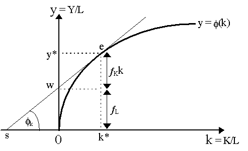
where y = Y/L and k = K/L. The intensive production function is depicted in Figure 4.
So what exactly are the income shares of capital and labor in Figure 4? At a given capital-labor ratio, the slope of the intensive production function is the marginal productivity of capital, i.e. f k = ¦ K. We also know that the marginal product of labor is thus the remainder, ¦ L = y - f kk (see our earlier discussion). Consider now the following procedure (originally due to Knut Wicksell (1893) and Joan Robinson (1956)). At a given capital-labor ratio, k*, the tangent line will have slope ¦ K, which is the marginal product of capital. Now, this tangent line crosses the vertical axis at point w in Figure 4. We claim now three things: (1) w is the real wage; (2) the portion on the vertical axis 0w are payments to labor per capita (w = ¦ LL/L = ¦ L); (3) the remaining portion on the vertical axis wy* are payments to capital per capita (wy* = ¦ KK/L). To see this, note that the following relationships hold in the diagram:
Consequently, ¦ KK/L = ¦ Kk* = wy*, i.e. per capita capital income is precisely the portion wy* on the vertical axis in Figure 4. As per capita labor income is y* - ¦ Kk, then consequently the rest of the vertical axis (portion 0w) is per capita labor income, ¦ L, thus w represents the real wage. Relative shares, ¦ KK/Y and ¦ LL/Y are obtained by dividing the per capita shares by the output-labor ratio, y*. Specifically, ¦ L/y = ¦ LL/Y and ¦ Kk/y = ¦ KK/Y. Thus, the relative income shares are obtained by calculating the relative sizes of the portions w and wy* on the vertical axis in Figure 4. What happens then when the capital-labor ratio changes? If k increases, y increases and so will w, the intercept of the tangent line on the vertical axis. But whether and how the relative shares of capital and labor change can be read diagramatically: if w rises more than y* rises, then the relative share of labor has risen relative to the share of capital. As Martin Bronfenbrenner (1960) has shown, the evolution of relative income shares depends in good part on the elasticity of substitution s . To see this formally, note that this question reduces to finding out whether ¦ KK/Y is positive or negative. This can be rewritten as ¦ Kk/y, thus differentiating with respect to k:
As y2 ³ 0 and y¦ KKk < 0, then in order to prove that the relative income share of capital rises with k, we must prove that:
or simply:
We write this in this manner because consultation with an earlier section ought to reveal that this is exactly the expression for the elasticity of substitution, s, in the constant returns to scale case in intensive form. Thus, for ¦ KK/Y to rise (fall) with k, then it must be that s > 1 (s < 1). To see this intuitively, recall that s is defined as:
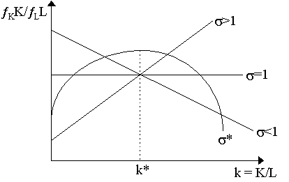
We can see how s captures the essence of this problem by trying to plot how relative income shares, ¦ KK/¦ LL change in response to a rise in the capital-labor ratio, k = K/L. A little bit of math will show that: 1/s - 1 = -¶ ln (¦KK/¦LL)/¶ ln (K/L) Various possible cases are depicted in Figure 5. Suppose s = 1, then the elasticity of substitution claims that ¦ K/¦ L and L/K rise proportionally, or, in other words, ¦ K/¦ L falls in exactly the proportion that K/L rises, thus ¦ KK/¦ LL is constant as K/L changes. This is shown by the horizontal line s = 1 in Figure 5. Suppose now that s > 1, then ¦ K/¦ L falls less than the amount K/L rises, thus ¦ KK/¦ LL rises when K/L rises. This is captured by the upward slope of the curve s > 1 in Figure 5. Finally, if s < 1, then ¦ K/¦ L falls more than the amount K/L rises, thus ¦ KK/¦ LL falls as K/L rises - thus the downward slope of the s < 1 curve in Figure 5.
The three curves s < 1, s = 1 and s > 1 depicted in Figure 5 assume that we have a constant elasticity of substitution production function, thus s is the same value throughout for any K/L. More generally, however, it is common to assume a relationship with varying elasticity of substitution, depicted by the hill-shaped locus s * in Figure 5: up to the capital-labor ratio k*, we have s > 1, at k*, s = 1 and after k*, s < 1. In this case, the relative shares of capital and labor vary differently with K/L depending on whether we are below or above the critical value k*. Thus, Bronfenbrenner's answer to Kaldor's "stylized fact" on constant relative income shares is that the elasticity of substitution tends not to stray from s = 1, thus relative income shares have remained constant. A second interesting hypothesis was laid out by David Ricardo (1817: Ch. 31), in his famous chapter "On Machinery" added to the third (1821) edition of the Principles. In effect, Ricardo had argued that the introduction of machinery would have an adverse effect on labor income. In our terms, the question is what is the impact of a rise in K on the absolute shares - and not relative shares - of income, i.e. the impact of K on rK and wL. (the issue of the impact of specific types of technical progress on relative income shares is discussed elsewhere). We shall concentrate mainly on the impact of a rise in K on rK. The specific question can be posed this way: does the amount of income going to capital increase if more capital is employed? The question can thus be written: when do we have it that ¶ (¦ KK)/¶ K > 0? Note that this is not self-evident: K increasing increases the numerator, but, as we know, substitution implies that ¦ K would fall, thus ¦ KK may rise or fall accordingly. By definition note that:
thus if this is to be positive, then it must be that:
as we are assuming that ¦ K > 0 and ¦ KK < 0. But notice that this is the inverse of the elasticity of the marginal product (i.e. capital demand) curve, i.e. -¦ KK·(K/¦ K) = e -1 where e = -(¶ K/¶ ¦ K)·(¦ K/K). Thus, if the demand for capital is elastic (i.e. e > 1), then the absolute income going to capital will rise with K; if demand for capital is inelastic (i.e. e < 1), then the absolute income going to capital will fall with K. This result, of course, is quite intuitive: elastic and thus relatively flat demand curve for capital means that a rise in K will reduce ¦ K very slightly, thus the income going to capital is bound to increase quite a bit; in contrast, an inelastic (and thus quite steep) demand curve for capital means that even a small rise in K will reduce ¦ K by a lot, thus capital income ¦ KK is bound to fall. It is easy to show that we can reduce this to a statement in terms of the elasticity of substitution. Recall that as ¦ (·) is homogeneous of degree one, then marginal products ¦ K(·) are homogeneous of degree zero, i.e. ¦ KKK + ¦ KLL = 0. Thus, ¦ KKK = -L¦ KL, so substituting into our earlier expression, we have:
as the necessary condition for a rise in K to increase ¦ KK. Now it is common to assume (and this is not implied) that ¦ KL > 0, thus we can rewrite this condition as:
or, multiplying by ¦ L/Y:
But again, by our earlier section we should recognize the term on the left as alternative form of the elasticity of substitution, s , for the constant returns to scale case. Thus, in order for a rise in K to increase ¦ KK we need:
i.e. the elasticity of substitution must be greater than the relative share of labor. Now, ¦ LL/Y < 1, so this is not enough to tell us much. But one thing should be recognized: it is entirely possible that ¦ LL/Y < s < 1. This means that it is possible that, when capital increases, that we simultaneously have it that the relative share of capital falls (as s < 1) while the absolute share of capital rises (¦ LL/Y < s ). Now we turn to the Ricardo question: does the amount of labor income rise or fall when machinery (K) is increased? This is read directly: ¶ ¦ LL/¶ K = ¦ KLL. If ¦ KL > 0, as has been assumed so far, then the absolute share of labor rises. Note the peculiarity in this result: whether labor income rises or falls when capital increases does not depend at all on what happens to the absolute share of capital, nor indeed on labor's own relative share. The amount of income received by a factor always rises when the quantity of the other factor increases. However, we must remind ourselves that this is rests on the ¦ KL > 0 assumption and is not implied by CRS or anything else. More details on the Neoclassical theory of distribution are found in our discussion of capital theory. A. Aftalion (1911) "Les Trois Notions de la Productivité et les Revenues", Revue d'Economie Politique. Vol. 25, p.145-84. E. Barone (1895) "Sopra un Libro del Wicksell", Giornale degli Economisti, Vol. 11, p.524-39. E. Barone (1896) "Studie sulla Distribuzione", Giornale degli Economisti, Vol. 12, p.107-55; 235-52. M. Bronfenbrenner (1960) "A Note on Relative Shares and the Elasticity of Substitution", Journal of Political Economy, Vol. 68, p.284-7. G. Cassel (1918) The Theory of Social Economy. 1932 edition, New York: Harcourt, Brace. S.J. Chapman (1906) "The Remuneration of Employers", Economic Journal, Vol. 16, p.523-28. J.B. Clark (1889) "Possibility of a Scientific Law of Wages", Publications of the American Economic Association, Vol. 4 (1) J.B. Clark (1891) "Distribution as Determined by a Law of Rent", Quarterly Journal of Economics, Vol. 5, p.289-318. J.B. Clark (1899) The Distribution of Wealth: A theory of wages, interest and profits. 1927 edition, New York: Macmillan. J.B. Clark (1901) "Wages and Interest as Determined by Marginal Productivity", Journal of Political Economy, Vol. 10. P.H. Douglas (1934) The Theory of Wages. New York: Macmillan. F.Y. Edgeworth (1904) "The Theory of Distribution" Quarterly Journal of Economics, Vol. 18, p. 149-219. F.Y. Edgeworth (1911) "Contributions to the Theory of Railway Rates, I & II", Economic Journal, Vol. 21, p.346-71, 551-71. A.W. Flux (1894) "Review of Wicksteed's Essay", Economic Journal, Vol. 4, p.305-8. J. Hicks (1932) The Theory of Wages. 1963 edition, London: Macmillan. J. Hicks (1934) "Marginal Productivity and the Principle of Variation", Economica, J.A. Hobson (1891) "The Law of the Three Rents", Quarterly Journal of Economics, Vol. 5, p.263-88. J.A. Hobson (1900) The Economics of Distribution. New York: Macmillan. J.A. Hobson (1909) The Industrial System. London: Longmans. W. Jaffé (1964) "New Light on an Old Quarrel: Barone's unpublished review of Wickseed's `Essay on the Coordination of the Laws of Distribution" and Related Documents", Cahiers Vilfredo Pareto, Vol. 3, p.61-102. As reprinted in D. Walker, 1983, editor, William Jaffé's Essays on Walras. Cambridge, UK: Cambridge University Press. N. Kaldor (1955) "Alternative Theories of Distribution", Review of Economic Studies, Vol. 23 (2), p.83-100. N. Kaldor (1961) "Capital Accumulation and Economic Growth", in F. Lutz and D. Hague, editors, The Theory of Capital, London: Macmillan. J.M. Keynes (1939) "Relative Movements of Real Wages and Output", Economic Journal, Vol. 49, p.34-9. M. Longfield (1834) Lectures on Political Economy. 1931 reprint, London: London School of Economics. F. Machlup (1937) "On the Meaning of Marginal Product", in Explorations in Economics in honor of Frank Taussig. New York: McGraw-Hill. T.R. Malthus (1815) Inquiry into the Nature and Progress of Rent. L. Makowski and J.M. Ostroy (1992) "The Existence of Perfectly Competitive Equilibrium à la Wicksteed", in Dasgupta, Gale, Hart and Maskin, editors, Economic Analysis of Markets and Games: Essays in honor of Frank Hahn. Cambridge, Mass: M.I.T. Press. A. Marshall (1890) Principles of Economics: An introductory volume. 1990 reprint of 1920 edition, Philadelphia: Porcupine. C. Menger (1871) Principles of Economics. 1981 edition of 1971 translation, New York: New York University Press. H. Neisser (1940) "A Note on the Pareto's Theory of Production", Econometrica, Vol. 8, p.79-88. V. Pareto (1896-7) Cours d'économie politique. 2 volumes. 1964 edition. V. Pareto (1902) "Review of Aupetit", Revue d'Economie Politique, Vol. 16, p.90-93. D. Ricardo (1815) An Essay on the Influence of a Low Price of Corn on the Profits of Stock. D. Ricardo (1817) The Principles of Political Economy and Taxation. 1973 of 1821 edition, London: Dent. Also reprinted in Volume I of Ricardo, 1951. D.H. Robertson (1931) "Wage Grumbles", in Robertson, Economic Fragments, London: P.H. King. As reprinted in American Economic Association, Readings in the Theory of Income Distribution. New York: Blakiston. J. Robinson (1934) "Euler's Theorem and the Problem of Distribution", Economic Journal, Vol. 44, p.398-414. J. Robinson (1956) The Accumulation of Capital. 1969 edition, London: Macmillan. G.B. Shaw (1928) The Intelligent Woman's Guide to Socialism and Capitalism. Garden City, NY: Garden City Publishing Co. H. Schultz (1929) "Marginal Productivity and the General Pricing Process", Journal of Political Economy, Vol. 37 (5), p.505-51. R.M. Solow (1957) "Technological Change and the Aggregate Production Function", Review of Economics and Statistics, Vol. 39, p.312-20. R.M. Solow (1958) "A Skeptical Note on the Constancy of Relative Shares", American Economic Review, Vol. 48, p.618-31. G.J. Stigler (1941) Production and Distribution Theories: The formative period. 1968 reprint, New York: Agathon. J.H. von Thünen (1826-50) The Isolated State, Vols. I & II. R. Torrens (1815) Essay on the External Corn Trade. F.A. Walker (1876) The Wages Question. 1881 edition, New York: Holt. F.A. Walker (1891) "The Doctrine of Rent and the Residual Claimant Theory of Wages", Quarterly Journal of Economics, Vol. 5, p.433-4. L. Walras (1874) Elements of Pure Economics: Or the theory of social wealth. 1954 translation of 1926 edition, Homewood, Ill.: Richard Irwin. L. Walras (1896) "Note on the Refutation of the English Law of Rent by Mr. Wicksteed", Appendix III to third edition of Walras, 1874. E. West (1815) Essay on the Application of Capital to Land. K. Wicksell (1893) Value, Capital and Rent. 1970 reprint of 1954 edition, New York: Augustus M. Kelley. K. Wicksell (1900) "Om gränsproduktiviteten sansom grundval för den nationalekonmiska fördelningen" ("Marginal Productivity as the Basis for Economic Distribution"), Eknomisk Tidskrift, Vol. 2, p.305-37, as translated in K. Wicksell, 1959. K. Wicksell (1901) Lectures on Political Economy, Vol. 1. 1967 reprint of 1934 edition, New York: Augustus M. Kelley. K. Wicksell (1902) "Till fördelningsproblemat" ("On the Problem of Distribution"), Ekonomisk Tidskrift, Vol. 4, p.424-33, as translated in K. Wicksell, 1959. K. Wicksell (1959) Selected Papers on Economic Theory, E. Lindhahl editor, R.S. Stedman translation, London: Allen & Unwin. P.H. Wicksteed (1894) Essay on the Co-Ordination of the Laws of Distribution. 1932 edition, London: L.S.E. P.H. Wicksteed (1910) The Common Sense of Political Economy. 1933 edition, London: Routledge and Kegan Paul. F. von Wieser (1889) Natural Value. 1971 reprint of 1893 translation, New York: Augustus M. Kelley.
|

All rights reserved, Gonçalo L. Fonseca