_________________________________________________________________
_________________________________________________________________ Contents (1) Pareto-Optimality The original constructors of the Paretian system were satisfied with the equality of the number of equations and unknowns to establish the existence of an equilibrium. Instead of pursuing this question more vigorously, their attention was turned onto something else: namely, suppose such a set of prices did exist, is the resulting equilibrium allocation an "efficient" one? By "efficiency" they referred to the concept of "Pareto optimality": i.e. a situation is Pareto-optimal if by reallocation you cannot make someone better off without making someone else worse off. In Pareto's words:
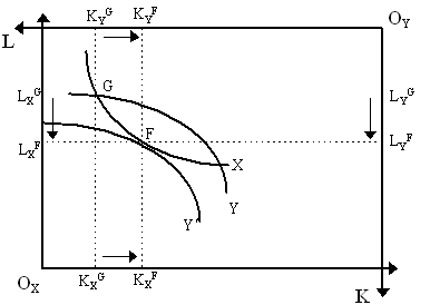
A situation is not Pareto-optimal, then, if you can make someone better off without making anyone else worse off. Clearly, as a concept of "efficiency", Pareto-optimality may seem quite adequate, but as a concept of "optimal", in any ethical sense, it is definitely not sufficient. As Amartya Sen (1970) notes, an economy can be Pareto-optimal, yet still "perfectly disgusting" by any ethical standards. It is thus of crucial importance to recall that Pareto-optimality, then, is merely a descriptive term, a property of an allocation, and that, at least a priori, there are no ethical propositions about the desirability of such allocations inherent within that notion. Thus, there is nothing inherent in Pareto-optimality that implies the maximization of social welfare (which shall be dealt with later). A second important note to recall is that Pareto-optimality is a general equilibrium notion and thus quite dependent on what we wish to include. For instance, two particular countries may have Pareto-optimal allocations within themselves, but when allowance is made for the trading opportunities that exist between both countries, the general allocation is no longer Pareto-optimal. Throughout this section, we alternate between the terms Pareto-optimality and Pareto-efficiency. Nonetheless, the term Pareto-efficiency is somewhat inadequate as some people naturally think of efficiency as a "technological" feature; but efficiency in production is only one part of what we mean. By "efficiency", in a Paretian context, we are required to also take into consideration "consumer efficiency". Thus, an economic situation can be "efficient" in a production sense, yet "inefficient" in a general Paretian sense. Pareto's own term, "maximum ophelimity", may not be a much better way of conveying the purely descriptive (and ethically neutral) meaning of the concept of Pareto-optimality. Perhaps the best description of Pareto-optimality is the underutilized one coined by Maurice Allais: an allocation is "Pareto-optimal" if there is an "absence of distributable surplus" (e.g. Allais, 1943, p.610). This is an excellent term as it conveys the true meaning of Pareto-optimality and suboptimality. One can think of a "distributable surplus" as the set of mutually beneficial (or at least not harmful) trades between any parties (firms, agents, countries, etc.) that have not been undertaken (e.g. the "lens" between indifference curves or isoquants in an Edgeworth-Bowley box constitutes a "distributable surplus"). By Allais's definition, if there is no distributable surplus, the situation is clearly Pareto-optimal. (A) Heuristics of Pareto-Optimality There are three important sets of efficiency conditions to be considered along the lines of the definitions provided by Pareto: (i) production efficiency; (ii) consumption efficiency; (iii) product mix efficiency. We shall consider each in turn. To visualize production efficiency diagrammatically, examine the situation in the Edgeworth-Bowley box in Figure 1 for our old two-sector model. At allocation G, the two firms are producing output levels X and Y. Although they are using factors fully, this an obvious "Pareto-inefficient" use of resources. For instance, we can reallocate factors between firms such that firm Y increases output from Y to Y¢ and firm X stays at the same level of output as before. Thus, moving from allocation G to allocation F is a Pareto-improving movement. In contrast, this new allocation, point F, is obviously a Pareto-efficient situation as any attempt to reallocate resources in order to increase output of one industry inevitably requires a reduction in output of the other industry. We can see immediately that, from the isoquants formed at an allocation, if there is a "lens" between the two isoquants, then we can undertake a Pareto-improving reallocation. Indeed, an allocation such as G will yield output levels that are in the interior of the production possibilities set (the area below the PPF). Thus, one of the first conditions for Pareto-efficiency is the familiar one that the marginal rates of technical substitution between any two factors be the same among all firms, in this case, MRTSXKL = MRTSYKL, which, in turn, implies that output combinations will be on the PPF.
While the equality of the MRTS is the central production efficiency condition in this two-sector context, there is another production efficiency condition which must be mentioned in light of its centrality in international trade theory. We have assumed, thus far in our examples, that there are two firms producing different outputs, X and Y. Suppose, however, that we have two firms (call them 1 and 2) both producing outputs X and Y. In this case, they each have their own (possibly different) PPFs and thus whatever output mix they produce will define their own marginal rate of product transformation between X and Y. The corresponding rule for efficiency in such case is that both firms produce output mixes where they have the same marginal rate of product transformation, i.e. MRPT1XY = MRPT2XY. This statement, of course, is merely the result of the theory of comparative advantage in international trade. Consider 1 and 2 to be different nations each producing two different goods, then production is efficient when each country specializes and trades (i.e. changes output combinations) until their MRPTXY are equal. If they are already equal, then no specialization is possible as the opportunity cost of good X in terms of good Y (i.e. MRPTXY) is the same in both firms/countries. We should note that Abba Lerner (1944) summarized production efficiency conditions in the following simple rule. Suppose we have F firms, n goods and m factors. Lerner proposed a general "transformation" function of the following form for the fth firm:
where xf = [x1f, x2, .., xnf] and an xif can be either an input or an output. Lerner's Rule, therefore, is that for any two firms, f, g = 1, 2, ..., F that:
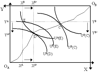
for any i, j = 1, 2, .., n+m. If xi is an output and xj is an input, then this equation states that the marginal product of xi should be the same for both firms. If both xi and xj is an input, then this states that the marginal rates of technical substitution between the inputs are the same for both firms (MRTSfij = MRTSgij). Finally, if xi and xj are both outputs, then this states that the marginal rate of product transformation are the same for both firms (MRPTfij = MRTSgij). In the post-war period, when differentiability was removed from Walrasian G.E., the corresponding conditions for production efficiency using merely convexity were established by Tjalling C. Koopmans (1951), which we have summarized elsewhere. Let us now turn to the second main condition for Pareto-optimality: consumption efficiency. The conditions for these are also clear enough and analagous to the first. In a consumer Edgeworth-Bowley box as in Figure 2 below, there are always gains to exchange unless the allocation is on the contract curve already. Thus, at allocation E (where A receives (XA, YA) and thus utility UA(E) and B receives (XB, YB) and thus utility UB(E)), we obviously have a Pareto-inferior allocation because one can always reallocate to improve utility of either agent without reducing anyone's utility level. For instance, if we trade some of agent A's allocation of Y with agent B's allocation of X, thereby moving from allocation E to allocation D, we obviously improve agent B's utility (which rises from UB(E) to UB(D)) without worsening agent A's (which stays at UA(E)). Allocation D is Pareto-optimal because we cannot undertake any further reallocations without hurting one of the agents.
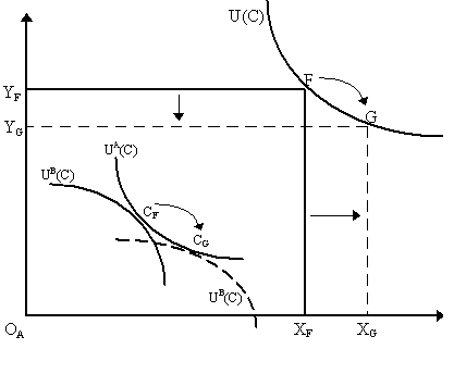
It is noticeable, from Figure 2, that D is Pareto-superior to E, but it is not the case that another Pareto-optimal allocation, such as C, is also Pareto-superior to E. In fact, C is not comparable to E by the Pareto criteria because one cannot go from initial allocation E to allocation C without hurting agent B (as his utility at C is lower than at E). Thus, while D is Pareto-superior to E, allocation C is not Pareto-comparable to either E or D. Note that the contract curve that connects origins OA and OB represent the set of Pareto-optimal allocations. Notice that, unlike the production case, we do not have a clear shape for the contract curve for consumers as we had for producers. Nonetheless, it is obvious that for consumption efficiency that an allocation between agents has to be Pareto-optimal and thus somewhere on the contract curve. Consequently, the second condition is that the marginal rate of substitution between two goods be the same among all consumers, thus for our particular example, MRSAXY = MRSBXY. The third condition for Pareto-optimality is that of product-mix efficiency: namely, that the marginal rate of substitution between two goods for any consumer be equal to the marginal rate of product transformation between those goods, i.e. MRSAXY = MRPTXY. Or, alternatively stated, that the marginal utility of good X with respect to Y equal the marginal cost of good X with respect to Y. The "efficiency" of this third condition may be less obvious at first, but it can be made clear via the use of the "community indifference curve" (CIC) or the "Scitovsky indifference curve" (SIC) as put forth by Tibor Scitovsky (1942). [note: the CIC was first introduced by Abba Lerner (1932) and made informal appearances in Wassily Leontief (1933), Jacob Viner (1937: p.521) and Tibor Scitovsky (1941).] Community indifference curves can be viewed in various ways. In their most ambitious interpretation, they are the upper contour set of a "community utility function", an index function of "aggregate utility". However, we shall resist this interpretation temporarily and refer to a particular CIC as a set of output combinations that yield the same "aggregate utility". We can see this diagrammatically in a simple two-sector model, as in Figure 3. Suppose we begin at point F which defines particular output levels, XF and YF which set the borders of an Edgeworth-Bowley box. Suppose, then, that there is some allocation of that output between the two individuals A and B such that MRSAXY = MRSBXY (point CF in the Edgeworth-Bowley box). Let us denote the utility levels achieved by agents A and B at point CF as UA(C) and UB(C). Thus, assuming comparability of some sort, we can argue that "aggregate" utility is some combination of the two utility levels, e.g. U(C) = UA(C) + UB(C). To trace out the CIC, we need to change the outputs X and Y such that the consumers stay at their same utility levels they had at C (and thus retain the same "aggregate" utility, U(C)). However, changing outputs X and Y changes the dimensions of the Edgeworth-Bowley Box. Clearly, if we see F as the origin of agent B, then changing output levels from F = (XF, YF) to G = (XG, YG) we are changing the agents B's origin from F to G. Consequently, the whole indifference map of agent B changes. Of course, the indifference map of agent A does not change as it is emanates from the bottom left origin, OA. Nonetheless, if the change in output is done carefully enough so that the utilities of agents A and B do not change, we need to somehow stay on agent A's indifference curve UA(C) and the tangency of that curve with the indifference map of agent B (at point CG) will yield an indifference curve for B that has exactly the same utility level as it had before (i.e. UB(C)). Thus, at output levels (XF, YF) and (XG, YG), agents A and B have the same utility levels, UA(C) and UB(C) that they had before. In this case, aggregate utility, U(C), is retained in the movement from F to G and thus we can say that F and G lie on the same "community indifference curve", U(C). It is a simple matter to note that the slope of the CIC curve at point F is the same as the slope of the individual indifference curves at point CF. Similarly, the slope of the CIC at point G is the same as the slope of the individual indifference curves at CG.
Scitovsky (1942) suggests that we consider the CIC the minimal levels of outputs X and Y that yield the same utility for each agent. As such, we can construct our CIC algebraically via a minimization problem. Specifically, given a fixed amount of X (call it X0), we wish to find the minimum level of Y so as to keep both agents at a particular utility level (say, UA(X, Y) = UA0 and UB(X, Y) = UB0). From consumption efficiency, we require that X = XA + XB and Y = YA + YB. Thus, we can set out a minimization problem as follows:
Setting up the Lagrangian:
which yields the first order conditions:
Combining the first two, we obtain UAX/UBX = m B/m A and the second two yield UAY/UBY = m B/m A, thus UAX/UBX = UAY/UBY, or simply:
i.e. the equality of the marginal rates of substitution for both agents. As these are merely the slopes of the indifference curves, then -dYA/dXA = UAX/UAY = UBX/UBY = -dYB/dXB, thus:
To find the slope of the CIC at the output levels (X0, Y0), recall that X0 = XA + XB and Y0 = YA + YB, so totally differentiating this last term:
so substituting in for dYA:
as dYA/dXA = dYB/dXB, then:
Thus, dividing through by the total differential for dX0:
or simply:
which states, quite simply, that the slope of the CIC curve is the equal to the slope of the indifference curve for agent A, i.e. MRSAXY. Thus, dY0/dX0 = MRSAXY = MRSBXY. A more general method of deriving the CIC can be found in Ivor Pearce (1964). The CIC curve that is constructed for a particular level of utility U(C), however, is not the only CIC curve that can be constructed that passes through point F. In the same Edgeworth-Bowley box - and thus at the same levels of X and Y - we can construct a different CIC curve by considering a different level of aggregate utility. Consider Figure 4. We see that in the Edgeworth-Bowley box constructed from point F, we have isolated two points of allocation, C and D, each yielding different levels of individual and aggregate utility. From point C, we have U(C) = UA(C) + UB(C) and thus are able to construct CICC corresponding to that aggregate utility level, U(C). From point D, we have U(D) = UA(D) + UB(D) from which we construct CICD corresponding to aggregate utility level U(D). Obviously, it is generally true that U(D) ¹ U(C) as the components of each are different. But as both U(D) and U(C) are attainable from allocations within the Edgeworth-Bowley box emanating from point F, then both CICC and CICD pass through F.
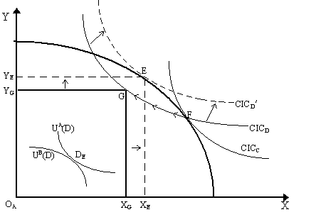
There is no reason to assume that CICC and CICD have the same slope - indeed, as long as the indifference curves of both agents within the Edgeworth-Bowley box have different MRSs at points C and D, then CICC and CICD will necessarily have different slopes at point F and, thus, intersect each other. These different slopes of the CICC and CICD curves at point F are captured by examining the price lines tangent to CICC (with slope -(pX/pY)C - which is also tangent to the MRSs of the agents at point C) and CICD (with slope -(pX/pY)D - which is also tangent to the MRSs at point D). This is obvious in Figure 4. As we can immediately envision, as there are an infinite number of allocations along a contract curve from F to OA representing different tangencies, there consequently could be an infinite number of CIC curves that pass through point F. Intersecting CIC curves are not troublesome, unless we wish to visualize the CICs as representing a social indifference mapping over outputs - as social welfare theorists would later endeavour to do. For our purposes, however, this intersection property is not troublesome. However, already a few things can be detected from close examination of Figure 4. Notice that CICC is tangent to the PPF while CICD is not tangent to it. Now, both CICC and CICD represents different aggregate utility levels and, at least from the outset, we cannot tell which one is superior because of their intersecting properties. However, we ca note that CICc represents a Pareto-optimal allocation whereas CICD does not. To see this, suppose we are at output combination F and our allocation of that output among households is at point D so that we are faced with CICD at point F. Turning now to Figure 5, we can move along the CICD curve to point G without reducing anyone's utility (as we saw before, everywhere along the CICD, the utility levels of agents are unchanged, at UA(D) and UB(D) respectively). At the new point G, we form a new Edgeworth-Bowley box with size XG and YG and the origin of agent B at G. Yet, note that G is in the interior of the production possibilities set and thus it represents an inefficient point. In other words, it is not true at G that the MRTSKL for both outputs are the same. Consequently we can expand output outwards from point G to point E, thereby expanding outputs from XG to XE and YG to YE. This will increase the utility of agent B (as his "distance from the origin" is greater, and thus the utility he attains at allocation D is greater than before) while not affecting the utility of agent A (still at UA(D)). In short, by moving from G to E, we have undertaken a Pareto-improving allocation. This is represented graphically in Figure 5 as an upward shift in the CICD curve to a new, higher level of aggregate utility, CICD¢ .
In sum, as we could undertake a Pareto-improving reallocation from the original point F to point E, then point F could not have been a Pareto-efficient allocation. However, this result depends crucially on the fact that CICD was not tangent to the PPF at point F. If we had instead an allocation in the Edgeworth-Bowley box such that we had CICC at point F, which is tangent to the PPF, then we immediately that a Pareto-improving reallocation is not possible. Thus, the third condition for Pareto-optimality, that MRSXY = MRPTXY makes perfect sense as MRSXY is the slope of the CIC curve at any output combination. [Incidentally, the set of outputs that yield Pareto-superior allocations to a particular output combination is known as the "Scitovsky set". Thus, in Figure 5, the Scitovsky sets of points F and G are merely the set of outputs above CICC and CICD respectively. Thus, any CIC can be seen merely as the lower boundary of the Scitovsky set defined at a point.] (B) General Pareto-Optimality Conditions Let us now turn to specifying the conditions for Pareto-optimality in a general economy with H agents, F firms, n goods and m factors. The notation is the same as the one used before. Thus, xh is a vector of commodities demanded by household h, xf is a vector of commodities supplied by firm f, vh is a vector of factors supplied by household h and vf is a vector of factors demanded by firm f. A particular household's utility depends on the amount of produced goods consumed and factors supplied, thus Uh(xh, vh) is household h's utility. A particular firm f faces an implicit production function of the form, F f(xf, vf) = 0. Following Oskar Lange (1942), we proceed to establish the conditions for Pareto-optimality in such a context by the maximization of a particular agent's utility (call him agent H) while keeping other all other agents' utility constant (thus Uh(xh, vh) = Uh0 for every h = 1, .., H-1, where Uh0 is some arbitrary setting), all firms are within their technological constraints (thus F f(xf, vf) = 0 for all f = 1, .., F), and assuming all resources are fully used (thus, total demand for commodities by households equal total supply of commodities by firms, i.e. å h=1H xih = å f=1Fxif for all i = 1, .., n and total demand for factors by firms equal total supply of commodities by households, i.e. å h=1H vjh = å f=1Fvjf for j = 1, .., m). Thus, the maximization problem is then:
Setting up the Lagrangian:
where mh, h = 1, .., H-1 are the Lagrangian multipliers for the households, mf, f = 1, .., F are the multipliers for the firms, and mi, i = 1,..., n and mj, j = 1, .., m are the multipliers for the goods and factor constraints respectively. The first order conditions for a maximum are as follows: for commodities,
and for factors,
and finally, for the multipliers:
These are the general conditions for Pareto-optimality. To connect with our more familiar heuristic forms, we can solve for m i/m k where i and k are two commodities (i, k = 1, 2, .., n) so:
This states that the marginal rates of substitution between any two produced goods, for any household h (including the Hth), must be equal to the ratio of the Lagrangian multipliers, m i/m k and thus each other. This is our familiar consumption efficiency condition for any two goods, i, k = 1, ...., n. Similarly, we can see that:
thus. the marginal rate of product transformation between goods i and k must be equal for every firm f = 1, .., F, part of the production efficiency conditions. Notice also that combining this with our previous condition, we see that for any f = 1, .., F and any h = 1, .., H, we have it that (¶ F f/¶ xif)/(¶ F f/¶ xif) = m i/m k = (¶ Uh/¶ xih)/(¶ Uh/¶ xkh), thus the marginal rate of product transformation between goods i and k for firm f is the same as the marginal rate of substitution between goods i and k for agent h - the familiar efficiency in product mix condition applied to any firm and household for any pair of goods, i, k = 1, .., n. Let us now turn to the factors. The conditions for these imply that for any two factors, j and q (j, q = 1, .., m) we have it that:
thus the marginal rate of substitution between factor supplies j and k are equal for all households (including the Hth). This is the factor supply analogue of the consumer efficiency condition, which we did not see diagramatically before. However, we can think of factor supply as own-consumption demand, e.g. leisure is the own-consumption of labor, and thus see its analogy to consumer efficiency conditions for own-consumption. Similarly, for any pair of factors j, q = 1, .., m, we have it that:
which states that the marginal rate of technical substitution between factors j and q must be equal for every firm, f = 1, .., F. This is our familiar production efficiency condition. We can combined it with our household factor supply condition so that for any f = 1, .., F and any h = 1, .., H, we see that (¶ F f/¶ xjf)/(¶ F f/¶ xqf) = m j/m q = (¶ Uh/¶ vjh)/(¶ Uh/¶ vqh), thus the marginal rate of technical substitution between factors j, q for firm f is the same as the marginal rate of substitution between factors j, q for household h. This is the factor-side version of the efficiency in product mix condition. Finally, we can notice that the following also holds for any commodity i = 1, .., n and any factor j = 1, .., m:
i.e. the marginal rates of substitution by household h between a factor j and a commodity i must be equal to the marginal rate of transformation of factor j into commodity i by firm f. Notice that this last is merely ¶ xif/¶ vjf, the marginal product of the jth factor in the ith output. Thus, this implies that marginal products (of a particular factor into a particular good) must be the same across all firms. If we think of factor j as labor and good i as bread, then marginal product of labor in bread production is equal among all firms and it is equal to ratio of marginal utilities of bread and labor for every household. (2) The Fundamental Welfare Theorems The Fundamental Theorems of Welfare Economics are deservingly famous as they link the concept of a competitive equilibrium with that of a Pareto-optimal allocation. Recall that the three crucial conditions for Pareto-optimal allocations in a Paretian system, as laid out explicitly by Abba Lerner (1934, 1944) and Harold Hotelling (1938) are the following:
As we can see these three conditions are similar to the conditions for equilibrium we stated earlier. In fact, they are (almost) identical. The two Fundamental Theorems of Welfare Economics, which stretch back to Pareto (1906) and Barone (1908), can thus be stated as follows:
The First and Second Welfare Theorems were proved graphically by Abba Lerner (1934) and mathematically by Harold Hotelling (1938), Oskar Lange (1942) and Maurice Allais (1943: p.617-35) (see also Abba Lerner (1944) and Paul Samuelson (1947)). Graphically, the basic idea of the First Theorem is simple: as we saw in our discussion of equilibrium in the Paretian system, if we have a competitive equilibrium, all three of the Pareto-optimal conditions are met. The Second Welfare theorem is almost equally clear intuitively: any Pareto-optimal allocation fulfills the three conditions, thus assuming differentiability, we can place price lines with slope pX/pY between the indifference curves so that MRSXYA = pX/pY = MRSBXY, place the same price line with the same slope between the CIC and the PPF so that MRSAXY = pX/pY = MRPTXY and, it must be that we are on the PPF (by production efficiency), then we can place a factor price line with slope r/w between the isoquants of the production Edgeworth-Bowley box so that MRTSXKL = MRTSYKL. Of course, the series of price lines we are inserting in this case may not correspond to the budget constraints of households properly speaking as we are only determining their slopes and not their precise location - which depends on endowments. Thus, the Second Welfare Theorem requires that we "adjust" the budget constraints (i.e. reallocate endowments) so that, upon utility-maximization, the resulting allocations will be equivalent to the Pareto-optimal one we are trying to reach. The Lange (1942)-Allais (1943) proof generalizes this idea to multiple commodities, factors, households and firms, but the essential idea is similar to this graphical intuition. Recall that we were given the multipliers, m i, i = 1, .., n for commodities and m j = 1, ..., m for factors. It is a simple matter to note that in the general equilibrium of a Paretian system, for all commodities i, k = 1, .., n, we have it that pi/pk = (¶ Uh/¶ xih)/(¶ Uh/¶ xkh) = (¶ F f/¶ xif)/(¶ F f/¶ xkf), for all household h = 1, ..,H and firms f = 1, .., F. Similarly, for all factors, j, q = 1, .., m we have it that wj/wq = (¶ F f/¶ vjf)/(¶ F f/¶ vqf) for all firms, f = 1, .., F and so on. The implication, then, is that if the multipliers are equal to prices, so, m i/m k = pi/pk and m j/m q = wj/wk, then the conditions for a Pareto-optimum and a competitive equilibrium in a Paretian system are identical. Thus, the conditions are equivalent in this sense. Of course, we must allow for corner solutions to the equilibrium problem, which that we obtain inequalities rather than equalities via the Kuhn-Tucker conditions; however, it is not difficult to generalize the Pareto-optimality conditions to allow for corner solutions by allowing for free goods, etc. Finally, these conditions all require the differentiability of utility functions and production functions, a condition which may be seen as unreasonable. Kenneth J. Arrow (1951) and Gerard Debreu (1951, 1954) extended these Fundamental Theorems without requiring differentiability and relying instead upon convexity and the separating hyperplane theorem - and thus we refer to our account of these. _________________________________________________________________ Maurice Allais (1943) Traité d'Economie Pure, 1952 edition of A la Recherche d'une Discipline Economique, Paris: Impremerie Internationale. Maurice Allais (1989) La Théorie Générale des Surplus. Grenoble: Presses Universitaires de Grenoble. Originally published in Économies et Sociétés, 1981, Nos. 1-5. Enrico Barone (1908) "The Ministry of Production in the Collectivist State", Giornale degli Economisti, as translated in Hayek, 1935, editor, Collectivist Economic Planning, London: Routledge. Francis M. Bator (1957) "The Simple Analytics of Welfare Maximization", American Economic Review, Vol. 47, p.22-59. Gottfried von Haberler (1933) The Theory of International Trade: with its applications to commercial policy. 1937 translation, New York: Macmillan. H. Hotelling (1938) "The General Welfare in Relation to Problems of Taxation and of Railway and Utility Rates", Econometrica, Vol. 6, p.242-69. Oskar Lange (1942) "The Foundations of Welfare Economics", Econometrica, Vol. 10 (3), p.215-28. W. Leontief (1933) "The Use of Indifference Curves in the Analysis of Foreign Trade", Quarterly Journal of Economics, Vol. 47, p.493-503. Abba P. Lerner (1932) "The Diagrammatical Representation of Cost Conditions in International Trade", Economica, Vol. 12, p.346-56. Abba P. Lerner (1934) "The Concept of Monopoly and the Measurement of Monopoly Power", Review of Economic Studies Abba P. Lerner (1944) The Economics of Control: Principles of welfare economics. New York: Macmillan. Vilfredo Pareto (1906) Manual of Political Economy. 1971 translation of 1927 edition, New York: Augustus M. Kelley. Ivor Pearce (1964) A Contribution to Demand Analysis. Oxford, UK: Oxford University Press Paul A. Samuelson (1947) Foundations of Economic Analysis. 1983 edition. Cambridge, Mass: Harvard University Press. Tibor Scitovsky (1941) "A Note on Welfare Propositions in Economics", Review of Economic Studies, Vol. 9, p.77-88. Tibor Scitovsky (1942) "A Reconsideration of the Theory of Tariffs", Review of Economic Studies, Vol. 9, p.89-110. J. Viner (1937) Studies in the Theory of International Trade. New York: Harper. _________________________________________________________________
|

All rights reserved, Gonçalo L. Fonseca