|
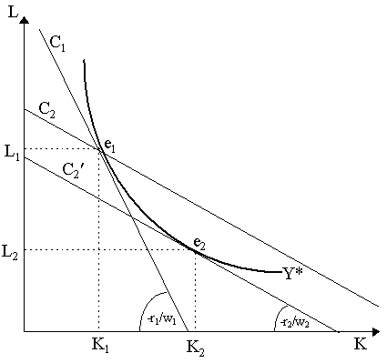
Contents (A) The Cost Function The cost-minimizing choice of inputs depended on two essential sets of parameters: the given output level (Y) and the given factor prices (r and w). It is obvious that if we changed relative factor prices, the cost-minimizing choice of inputs would change. Consider Figure 8.1 At factor price r1/w1, the cost-minimizing input choice is K1, L1, represented by point e1, at the tangency of the C1 isocost curve and the Y* isoquant. Now, suppose that the rental rate of capital fell and the wage level rose, so that the isocost curve at e1 is now C2, which has slope -r2/w2, where r2/w2 < r1/w1. Obviously, e1 no longer represents the cost-minimizing input choice. Instead, the cost-minimizing producer would prefer to change technique and move to a point such as e2, at the tangency of the isocost curve C2¢ and the isoquant Y*. The new choice of inputs, K2, L2, is considerably different: namely, more capital and less labor will be hired at e2, relative to before.
Points e1 and e2 in Figure 8.1 both represent cost-minimizing points, albeit at different factor prices. However, one question remains: in the move from e1 to e2, have costs risen or fallen? This we cannot tell directly from the picture in Figure 8.1, as the isocost curves C1 and C2¢ are not obviously comparable. However, in principle, they should be: C1 are the total costs at e1 at the old prices r1/w1, while C2¢ are the total costs at e2 at the new prices, r2/w2. Both C1 and C2¢ are numbers, thus we should be able to say whether total costs at e1 are higher or lower than total costs at e2 depending on whether C1 is greater or less than C2¢ . Consequently, we should be able to say whether factor prices r1/w1 yield higher or lower total costs than factor prices r2/w2 by comparing the relevant costs at their respective cost-minimizing points, in this case, C1 and C2¢ . Thus, we can trace out what can be called a minimum cost function (or simply, a cost function), C = C(r, w, Y*), representing the different minimum costs yielded by different factor price and output configurations. As noted, these costs are evaluated at the relevant cost-minimizing choice of inputs, thus C1 and C2¢ in Figure 8.1 would be included in the cost function, but C2 would not. Of course, the output level Y* one of the parameters of the cost-minimization story, must be included in the cost function. Its inclusion helps us connect the cost function from the cost-minimization Paretian story with the cost function of the scale-theoretic Marshallian story. However, we shall postpone the Marshallian themes (e.g. long run versus short-run cost functions), and just outline some of the properties of the cost function we have here. For generality, we shall rewrite the cost function simply as C = C(w, y), where w represents a vector of factor prices and y represents the given level of output. In this way, the cost function can be written as:
where V(y) is the input requirement set formed by the isoquant of the desired y. The cost function and its analysis is due largely to the famous work of Paul Samuelson (1947) and Ronald Shephard (1953) [note: John Hicks (1939) obtained most of these relationships in the context of a consumer expenditure function]. Its general properties are the following:
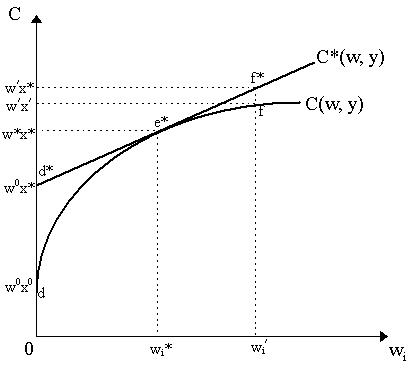
The explanation of these properties are easily enumerated. Property (1) simply states that in order to produce positive output (y > 0) and if factors are not free, then costs will be incurred. Property (2) states that the cost-minimizing choice of output to produce nothing will cost nothing. Notice that this is equivalent to saying that there are no fixed costs, i.e. costs incurred before one even begins producing. Property (3) is straightforward enough: if the required level of output rises (i.e. isoquant Y* shifts up to the northeast), then, everything else constant, the total costs incurred at the cost-minimizing point will be higher. Property (4), which claims that increasing any one factor return will increase costs can be deduced by simple revealed choice reasoning. Let w and w¢ be two factor price vectors such that w¢ ³ w. Suppose that at factor prices w, x was the cost-minimizing input choice (thus, C(w, y) = wx) while at price w¢ , x¢ was the cost-minimizing input choice (thus C(w, y) = w¢ x¢ ). Now, as w¢ ³ w, then at factor prices w, when x was chosen, x¢ might have also been available but it was not chosen. This implies that wx £ wx¢ , otherwise x would not have been the cost-minimizing choice of inputs. But as w¢ ³ w, then we have wx¢ £ w¢ x¢ . Thus, combining inequalities, we see that wx £ w¢ x¢ , which translates to C(w, y) £ C(w¢ , y). Thus, inequality (4). Property (5), which establishes the homogeneity of degree 1 of the cost function (doubling all factor prices, doubles total costs), is also straightforward. Suppose, in our canonical example, we increased both factor prices r and w by the scalar l . Then costs change from C = wL + rK to C¢ = l wL + l rK. If L and K do not change, then we see immediately that C¢ = l C. However, it is evident that L and K will not change. Specifically, recall that the slope of the isocost function is -r/w. Increasing both prices by the scalar l , the slope remains unchanged as -l r/l w = -r/w. Thus, the cost-minimizing choice of inputs, L and K, will not change. Thus, the only thing that changes are the numerical value of total costs, which rise from wL + rK = C to l wL + l rK = l C. Thus, the homogeneity of the cost function. Property (6), the concavity of the cost function, can be understood via the use of Figure 8.2. We have drawn two cost functions, C*(w, y) and C(w, y), where total costs are mapped with respect to one factor price, wi. All other factor prices and the output level are being held constant. Suppose that we have Leontief, no-substitution production technology, so that the cost-minimizing point is always a particular input combination, call it x*, regardless of the factor prices. The corresponding cost function is shown in Figure 8.2 by C*(w, y). Now, because of our Leontief technology, we have a fixed cost-minimizing bundle x* throughout, so as we increase the rental rate of the ith factor, wi, the total costs of the bundle increase linearly. This becomes obvious when we note that the cost of the bundle x* at any particular set of factor prices w is:
where wixi* are the total payments to the ith factor and å j=1m-1wjxj* are the payments to the other factors. Thus, increasing only wi will increase total costs wx* linearly, thus C*(w, y) is a linear function, as depicted in Figure 8.2.
Now, suppose that the rental rate of ith factor is zero, wi = 0. Although the ith factor may be free (so wixi* = 0), the other factors are still costly (å j=1m-1wjxj* > 0). Thus the costs of producing bundle x* are positive, i.e. w0x* > 0, as shown by point d* in Figure 8.2. As the rental rate of the ith factor increases, the costs of bundle x* increase linearly. As we see in Figure 8.2, when wi = wi*, costs are w*x* (point e*) and when wi = wi¢ , costs are w¢x* (point f*). Now, let us increase the degree of substitutability, i.e. let us move away from the Leontief technology and allow there to be different cost-minimizing input bundles at different factor prices. We propose that the new cost function will actually look like the concave function C(w, y) in Figure 8.2. To see why, let us suppose that when we have factor prices w* (and thus wi = wi*), then the old bundle x* is still the cost-minimizing bundle. Thus, w*x* is cost-minimizing, thus both the old cost function C*(w, y) and the new one C(w, y) share point e* in Figure 8.2. However, from point e*, let us suppose the price of the ith factor rises from wi* to wi¢ . In the old cost-function, where Leontief technology forced the producer to be stuck with input bundle x*, all that would happen would be that costs would increase from w*x* to w¢ x*. However, now that there is a degree of substitability, producers will seek another cost-minimizing bundle x¢ . It should be obvious that the costsof the new cost-minimizing bundle are not going to be more than the costs incurred if the producer could not choose a new bundle. In other words, w¢ x¢ £ w¢ x* thus, as shown in Figure 8.2, point f lies below f*. This reflects the very simple idea of subtitutability: when given the choice, the producer will choose an input combination x¢ with lower costs than x* by substituting away from the factor whose costs have risen (in this case, the ith factor). Thus, at least for wi > wi*, the cost function C(w, y) will lie below the Leontief cost function C*(w, y). An analogous reasoning applies for points below wi < wi*. Thus, the general concavity of the cost function, C(w, y). Let us turn to a formal demonstration. Let w, w¢ be two factor price vectors and let x and x¢ be the corresponding cost-minimizing factor bundles. Let us define w0 = l w + (1-l )w¢ , where l Î (0, 1), thus w0 is a convex combination of factor prices w and w¢ . Consider now another input factor bundle, x0 which is cost-minimizing at prices w0. By the convexity of the isoquants, it is obvious that x0 was available at the other factor prices w and w¢ , but was not chosen at those prices. Thus, by cost-minimization, the following inequalities hold for factor prices w and w¢ :
Multiplying the first by l and the second by (1-l ), and then adding the inequalities, we see immediately that:
by definition. But as wx = C(w, y), w¢ x¢ = C(w¢ , y) and w0x0 = C(w0, y), then we see immediately that this inequality translates into:
Or, more obviously:
thus implying that the cost-minimizing function C(·, y) is concave in w. Thus, Property 6. Property 7 follows simply by the assumption of the convexity of the isoquants and linearity of the cost function: as factor prices change continuously, there is continuous substitution along the isoquants and by linearity, the costs change continuously. Property 8 is the famous Shephard's Lemma, ¶ C(w, y)/¶ wi = xi. A simple proof employs the envelope theorem. Total costs are C(w, y) = w·x = å i=1m wixi. Taking the total derivative with respect to wi, we obtain:
(recall that wj are given, thus they do not change with respect to wi). We want to apply the envelope theorem, which will basically make the entire summation term disappear and leave only xi. Now, recall that xj is the solution to the cost-minimization problem, thus recall that the first order condition implies that wj = l ¦ j. Now, recall also that we required that at the solution, y* = ¦ (x). Differentiating this with respect to wi, we obtain:
As the first order condition implies ¦ j = wjl for all j = 1, 2, .., m, then we can rewrite this as:
which, if l is non-zero and finite, implies that the entire summation term in our earlier equation is zero. Thus, ¶ C(w, y)/¶ wi = xi, which is what was sought. [Note: although named after Shephard (1953), who gave a complete proof using the distance function, we nonetheless see it in John Hicks (1939: p.331) and Paul Samuelson (1947: p.68)] The reasoning can be restated intuitively this way: suppose that given factor prices w, the bundle x is the cost-minimizing bundle. Increasing the price of the ith factor marginally (i.e. by one dollar) and allowing for no substitution so that the x remains the cost-minimizing bundle (the implication of the envelope theorem), then it is obvious that the total costs of the bundle will increase only by the amount which spending on the ith factor increases. Now, at the previous factor prices w, we were spending wixi on the ith factor. Consequently, a rise in factor prices by a dollar, will raise total costs by xi. More heuristically, if at prices w, wi = $5 and xi = 100, then total expenditure on the ith factor was wixi = $500. Increasing wi from $5 to $6 without changing the bundle (so xi = 100 still), then we now have total expenditure wi¢ xi = $600. Thus, the change in expenditure on the ith factor when we increased factor prices by a dollar is $100, i.e. precisely the amount of the xi factor employed, converted to dollars. Thus, ¶ C(w, y)/¶ wi = 100 = xi. (B) The Derived Demand for Factors In the cost-minimization and output-maximization exercises, we were able to determine the input combinations chosen by the producer. We noticed that the choice of input combinations depends on two sets of parameters - the factor prices (w) and the desired output level (y). Consequently, we can define the input combinations chosen by the firm in response to factor prices and the desired output levels as the compensated demand for factors. Specifically, these demand functions are merely the arguments that minmize the cost function, so they can be written succinctly as:
where V(y) is the input requirement set of the desired y. One must remember that x(p, w) is a vector of functions, thus the demand for a particular factor xi(p, w) is merely one of the entries. The producer's demand for the ith factor, xi(p, w), is a function of rental rates and the desired output level. For our canonical case, we would infer from the first order conditions a function Kd = K(r, w, Y*) as capital demand function and Ld = L(r, w, Y*) as the labor demand function of the producer. What are the properties of these factor demand functions? In particular, what happens to factor demands when particular input prices or output levels change? The major tool for this is Shephard's Lemma, which stated that ¶ C(w, y)/¶ wi = xi. This resulting xi is precisely the demand for the factor i at factor prices w and output level y. Thus, by Shephard's Lemma, we can analyze the properties of the factor demand functions merely by examining the properties of the first derivative of the cost function. We shall be doing this throughout. We can delineate the factor price properties of the compensated factor demand functions as follows:
Property (1) is the basic proposition that the factor demand curve is downward-sloping, i.e. a rise in the price of a factor will lead to a decline in the demand for it. Diagramatically, we have already seen in Figure 8.1 when we reduced the factor price ratio r/w, the cost-minimizing input bundle moved from e1 (high labor, low capital) to e2 (low labor, high capital). In other words, we saw that as the wage rose relative to the rental rate on capital, the demand for labor fell while the demand for capital rose. Thus, at least in the simple diagrammatic case of Figure 8.1, an increase in the factor price will lead to a fall in the demand for that factor by the producer. To prove this more generally, consider first the impact of a change in the rental rate of the ith factor on that demand for for that factor, i.e. ¶ xi(w, y)/¶ wi. Applying Shephard's Lemma we should recognize immediately that as xi is the partial derivative of the cost function with respect to wi, then ¶ xi/¶ wj is the second partial derivative of the cost function, i.e.
Now, recall that one of the properties of cost functions were their concavity with respect to individual factor prices. This implies that ¶ 2C(w, y)/¶ wi2 £ 0, thus:
so that a rise in the ith factor price will reduce the demand for that factor, precisely the result we obtained diagramatically in Figure 8.1. Property (2) follows by virtually the same logic. As by Shephard's Lemma ¶ xi(w, y)/¶ wj = ¶ 2C(w, y)/¶ wi¶ wj. Now, Young's Theorem tells us that ¶ 2C(w, y)/¶ wi¶ wj = ¶ 2C(w, y)/¶ wj¶ wi. But we know by Shephard's Lemma that ¶ 2C(w, y)/¶ wj¶ wi = ¶ xj(p, w)/¶ wi. Thus:
i.e. in the margin, the effect of a rise in price of factor j on the demand for factor i is the same as the effect of a rise in the price of factor i on the demand for factor j. This symmetry of cross-effects is not very economically intuitive, but it follows through. However, although cross-price elasticities are not symmetric. Specifically, we can define the elasticity of demand for factor i with respect to price of factor j as:
Our previous result implies that e ii £ 0, so own-price elasticity is negative. But generally e ij ¹ e ji. This is evident because e ji = (¶ xj/¶ wi)·(wi/xj), so e ij = e ji only if wj/xi = wi/xj, which we have no reason to assume. Nonetheless, notice that:
Thus by symmetry of cross effects e ij(xi/wj) = e ji(xj/wi), which implies that:
Defining sj = wjxj/C(w, y), which as we can note is the proportion of total costs spent on factor j and si = wixi/C(w, y), the proportion of total costs spent on factor i, then immediately we see that:
Thus the cross-price elasticities are proportional to each other, with the proportionality factor being sj/si, the ratio of relative shares of the two factor bills in total costs. It is a simple matter to note that e ij/sj is actually the good old Allen elasticity of substitution we derived earlier. Specifically, recall that we defined the Allen elasticity of substitution as:
where |B| is the determinant of the bordered Hessian matrix and |Bij| is the ijth cofactor for the production function y = ¦ (x1, x2, .., xm). To see the connection, note that from the first order conditions of the cost-minimization problem, we have wj = l ¦ j for j = 1, .., m and y = ¦ (x1, x2, .., xm). Thus, totally differentiating all the first order conditions with respect to l and all the xis:
can set up the result in matrix form as:
where, note, the matrix on the left is merely the bordered Hessian for a production function. Now, in order to derive ¶ xi/¶ wj for a particular wj and xi on a particular isoquant then we can set dwk = 0 for all k ¹ j (thus keeping all factor prices but the jth fxed) and set dy = 0 (thus staying on the same isoquant). Thus, the system of equations can thus be rewritten as:
where, note, we are interpreting the ratios dxi/dwj as partial derivatives, ¶ xi/¶ wj. Now, for a particular xi, in order to obtain ¶xi/¶ wj, we can apply Cramer's rule:
where |B| is the determinant of the Hessian matrix, while |Bij| is the determinant of the Hessian matrix with the column [0, 0, ..0, 1, 0, 0] replacing the ith column of B. Note that as we can expand by the ith column which is all zeroes expect for the jth component (which is 1), then |Bij| is actually the cofactor of the ijth element of the Hessian matrix, B. Now, multiplying ¶xi/¶wj by wj/xi, we obtain:
Thus, dividing by sj = wjxj/(å i=1m ¦ ixi), we obtain:
which is precisely the expression for the Allen elasticity of substitution, s Aij. Finally, turning to the result we obtained earlier that e ij = e ji(sj/si), this can be restated as e ij/sj = e ji/si, or s ijA = s jiA, so that the Allen elasticities of substitution are symmetric. Property (3) is somewhat clearer. Consider the impact of a change in all input prices by a particular scalar (call it l ). Diagramatically, we should expect (as we noted before) that the choice of inputs would remain unchanged - largely because a doubling of all prices will leave the slopes of the isocost curves unchanged. We can see this directly by remembering that the cost function is homogeneous of degree one, i.e. C(l w, y) = l C(w, y). But we know from earlier discussion that if a function is homogeneous of degree r, then its partial derivatives are homogeneous of degree r-1. By Shephard's Lemma, xi(w, y) is a first partial derivative of a C(w, y), thus demand will be homogenous of degree zero, i.e. xi(l w, y) = xi(w, y), doubling all factor prices will not affect the demand for any input. We can exploit this a bit further. By Euler's Theorem , if a function is homogeneous of degree zero, then the sum of the arguments multiplied by their partial derivatives will be zero, i.e.
Now, this identity is extremely useful. Note that multiplying the sum by 1 = xi/xi this can be rewritten:
which (if xi is finite and non-zero) implies:
so the sum of price elasticities of demand for factor i is equal to zero. Now, returning to the earlier identity, applying Shephard's Lemma we should recall that ¶ xi(w, y)/¶ wj =¶ 2C(w, y)/¶ wi¶ wj. Plugging this back into our Euler's Theorem equation:
or, more generally:
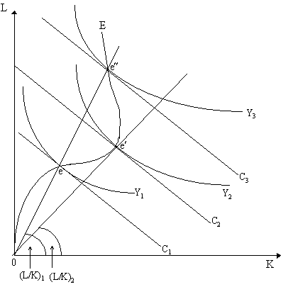
where ÑwwC(w, y) is a matrix of second derivatives of the cost function. The elements on the diagonal are the own-price effects on demands, while those on the off-diagonal are the cross-price effects. By what we have said before, concavity and Young's Theorem implies that Ñ wwC(w, y) will be a negative, semi-definite symmetric matrix. Let us now turn to changes in desired output, an issue we have been avoiding because of the close association of this theme to Marshallian theory. Cost functions C(w, y) are functions of output, and thus so are demand functions, x(w, y). The questions we are posing are illustrated in Figure 8.3. At a particular desired output level Y1, the cost-minimizing bundle is e. Suppose now that desired output increases to Y2. As factor prices are unchanged, it is obvious that conducting the same cost-minimizing exercise, we obtain optimal input bundle e¢ . If output rises again to Y3, then the cost-minimizing input bundle is e¢¢ .
As output increases from Y1 to Y2 and Y3, we change the cost-minimizing bundle from e to e¢ and e¢¢ . The curve E passing through e, e¢ and e¢¢ in Figure 8.3 is referred to as the output-expansion path and traces the different cost-minimizing bundles as we change the level of output. Notice that the slopes of the isoquants at e, e¢ and e¢¢ are the same (all equal to the factor price ratio, the slope of the isocost curves). Obviously, the isocost curve C1 associated with the bundle e is below the isocost curve C2 associated with e¢ which, in turn, is below C3 associated with e¢¢ , i.e. C1 < C2 < C3. Thus, immediately we see that a rise in output will increase the costs associated with the cost-minimizing bundle, or ¶ C/¶ y ³ 0. What can we say about the effect of increasing output on factor demands? Diagramatically, in Figure 8.3, we saw that the demand for both capital and labor has increased. But this is not always obvious. Recognize that by Shephard's Lemma:
But by Young's Theorem, interchanging the terms in the denominator:
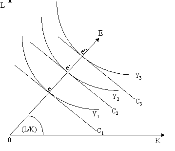
Now, as we saw, ¶ C/¶ y ³ 0 by the properties of the cost function. Now, ¶ C/¶ y can be interpreted as the marginal cost of output. Thus, whether an increase in output increases or decreases factor demands depends upon whether a rise in price of factor i increases or decreases the marginal cost of output. It is not clear what will be the sign of ¶ xi/¶ y. We would like it that ¶ xi/¶ y ³ 0 (as is implied in Figure 8.3). In such a case, we refer to the factor as a normal factor. But it can happen that ¶ xi/¶ y < 0, in which case we have an inferior factor. This might happen if, say, the factor was indispensible at low scales of production but is substituted against as higher levels of output are achieved. An argument that might justify this would appeal to phenomona such as specialization, indivisibilities, etc. Recall that we have already touched upon specialization arguments in our discussion of returns to scale of production functions. Specifically, we argued that differing returns to scale are often justified on the basis of changing factor proportions as output changed. However, we also spoke of pure returns to scale, a technical property of the production function summarized by the notion of "doubling all inputs, etc." It must be clear that now we are not talking about technical properties of scale but economic properties of scale. In other words, we are interested in cost-minimizing points as the output level increases. This may very well allow for changing factor proportions. We see this clearly in Figure 8.3. The labor-capital ratio at e, denoted by the slope of the ray from the origin (L/K)1, is different from the labor-capital ratio at e¢ , represented by the different ray from the origin (L/K)2. Thus, cost-minimization at different output levels can yield different factor proportions or techniques. Indeed, as long as the output expansion path E is curved in any way, there will be changing factor proportions as scale increases. Happily, the technical aspects of the production function may, in fact, restrict the type of output-expansion paths we see. Specifically, it can be shown that if the production function is homothetic (and all production functions which are homogeneous of whatever degree are homothetic), then there will not be changing factor proportions along the output-expansion path. In other words, the output expansion path E will necessarily be a ray from the origin. Such a situation is depicted in Figure 8.4, where the cost-minimizing points e, e¢ and e¢¢ all lie on the same ray from the origin, E, which also represents the output-expansion path.
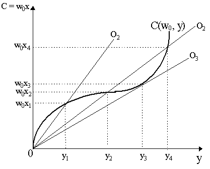
Thus, although in principle, output-expansion paths may be curved and twisted, most relevant production functions (which are usually homothetic) will nonetheless exhibit linear output expansion paths. Notice that linearity does not rely upon constant returns to scale. Increasing returns and decreasing returns production functions will also have linear expansion paths. Homotheticity of the production function buys us a few more things in this context: for instance, it guarantees that every factor is normal. (C) Costs and Returns to Scale As we have demonstrated, the cost function C(w, y) is positively related to the scale of output. However, as we saw in an earlier section earlier, a production function can exhibit different returns to scale. One ought to imagine that the cost function would thus also capture these different returns to scale in one way or another. This is shown in Figure 8.5 below, where we have plotted the cost function C(w0, y), where output is plotted with respect to y, and factor prices are held fixed at w0. As we see in Figure 8.5, as output increases, costs increase, but at different speeds. The easiest way to think of the shape of the cost curve in Figure 8.5 is to recall the typical varying returns-to-scale production function for the one-input, one-output case shown earlier in Figure 3.1. There our production function y = ¦ (x) exhibited first increasing and then decreasing returns to scale as output level rose. The cost function C(w0, y) drawn in Figure 8.5 is merely a "stretched mirror image" of the production function in Figure 3.1. In Figure 3.1, y was on the vertical axis and x was on the horizontal. Suppose we flip this around so that y is on the horizontal axis and x on the vertical. The resulting shape would be similar to the cost function in Figure 8.5. However, in Figure 8.5, we do not measure factor inputs on the vertical axis but rather costs. However, recall that costs are merely w·x. As factor prices are fixed throughout at w0, then all we need to do is take our inverted production function and "stretch" x by the scalar w0. Thus, the total function C(w0, y) in Figure 8.5 is merely the production function in 3.1 with axes flipped and the vertical axis increments reindexed from x to w0x.
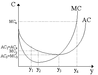
However, we do not have to restrict ourselves to production technology which is one-output, one-input. Indeed, a production function with multiple inputs y = ¦ (x1, x2, x3, .., xm) would be effectively the same as that depicted in Figure 8.5 because the the cost of a single bundle of factors x at a particular, fixed set of w0 would still be a single number, w0·x and thus the cost function corresponding to any multi-factor production function with increasing and then decreasing returns to scale could still be drawn on a plane as in Figure 8.5. The properties of increasing, constant and decreasing returns to scale correspond, when viewed from the perspective of the cost function, to decreasing, constant and increasing marginal costs to scale. As we see in Figure 8.5, costs increase as output increases throughout; however, notice that the cost function is first concave and then convex. If we define marginal cost of output as MC = ¶ C/¶ y, the slope of the cost function in Figure 8.5, then we see that marginal costs fall as we raise output from zero to y2 and then begin to rise as we move from y2 onwards. The marginal cost curve can thus be drawn independently, as we have done in Figure 8.6. Average costs can also be deduced. By definition, AC = C/Y, thus average costs at any point are captured by the slope of a ray through the origin that passes through it. As we see in Figure 8.5, average costs at y1 are high, and average costs at y3 are low as ray O1 is steeper than ray O3. Average costs at y2 and y4 are the same as they share the same ray, O2. Notice that O3 is the flattest ray we can obtain, thus y3 represents the output level with the lowest average cost. Thus, as we can deduce from Figure 8.5, average costs decline as output rises from zero to y3 and then rise again after that. The average cost curve is drawn also independently in Figure 8.6. The average cost and marginal costs curves are due originally to Jacob Viner (1931) and thus the curves in Figure 8.6 are sometimes referred to as Viner curves.
Notice that y2 is the inflection point in the cost function in Figure 8.5, thus y2 represents the point where we move from decreasing to increasing marginal costs, while y3 is where we move from decreasing to to increasing average costs. As y2 < y3, we can define several regions of output: in the region from 0 to y2, average costs and marginal costs are declining and AC > MC; in the region from y2 to y3, we still have AC > MC and average costs declining, but marginal costs are rising; from y3 onwards, we now have MC > AC and both average and marginal costs increasing. Notice that the MC and AC curves intersect at y3 which also happens to the be the point of minimum average cost and that everywhere below y3, MC < AC and everywhere above y3, AC > MC. This is obvious diagramatically, but can be proved algebraically. As AC = C(w, y)/y, then at output levels below y3 (i.e. when AC is declining), we must have ¶ (AC)/¶ y < 0. But this translates to by differentiation:
or, rearranging:
so multiplying through by y:
thus MC must lie below AC at output levels below y3. The analogous exercise can be done for points above y3 where AC is increasing. Returning to the relationship between returns and costs, it can be easily inferred from the diagram that different returns to scale correspond to different marginal costs (not average costs). Where we have increasing returns to scale, we have decreasing marginal costs (thus, between 0 and y2); where we have decreasing returns to scale, we have increasing marginal costs (above y2). Notice the implication: if we have a production function which has decreasing returns to scale throughout, then both our marginal and average cost functions are always rising; if it has increasing returns throughout, then both the marginal and average cost functions are falling throughout. Finally, a constant returns to scale production function necessarily implies flat AC and MC curves. Several other properties can be detected about marginal cost. Firstly, we have already deduced earlier that marginal cost is always non-negative, i.e. ¶ C/¶ y ³ 0. But we also ran into the difficulty that we could not unambiguously detect what happens to marginal cost when a factor price rises, i.e. we could not tell exactly what ¶ [¶ C(w, y)/¶ y]/¶ wi is because of possible substitution possibilities. However, what if all factor prices rise proportionally? We can establish the following interesting property: namely, that marginal cost is homogenous of degree one in prices, i.e.
so that a proportional rise in factor prices will lead to a proportional rise in marginal cost. To obtain this, we need to recall our result that C(w, y) is homogeneous of degree one in prices. This implies, by Euler's theorem, that:
consequently, differentiating with respect to y:
or as ¶ 2C/¶ wiyi = ¶ 2C/¶ yiwi by Young's Theorem, then:
But notice that this just says that marginal cost (¶ C/¶ y) can be expressed as a sum of its arguments (wi) multiplied by their derivatives (¶ (¶ C/¶ y)/¶ wi). Thus, by Euler's Theorem, ¶ C/¶ y is homogeneous of degree one, i.e. doubling all factor prices will double marginal costs. This fact caused a dilemma in early economic theory. Specifically, it commonly stipulated that it was an empirical fact (albeit rooted in armchair speculation) that agriculture exhibited decreasing returns to scale while manufacturing always exhibited increasing returns to scale. This idea can be found in the early work of the Classical economists. Alfred Marshall reiterates this idea:
The dilemma arises in that a firm whose technology exhibits increasing returns throughout implies that there are decreasing marginal costs throughout. If the technical returns to scale properties of the production function can be captured by the cost curve C(w0, y), can we also obtain the rest of the properties of the production function (e.g. convexity of the isoquants, etc.) via the cost function? Indeed, we can. As Hirofumi Uzawa (1964) has shown, one can obtain isoquants of the production function from the revaled cost-minimizing choices. Changing factor prices continuously for a given level of output, the cost-minimizing choices will trace out the corresponding isoquant of that level of output. Thus, even if we do not know the isoquants, we can hypothetically trace them out from the cost-minimizing choices of the producers. However, a caveat is in order: while we can recover convex isoquants by tracing the cost-minimizing points, we cannot recover non-convex isoquants by these means. In other words, if the true production function has non-convex input requirement set V(y), then by Uzawa's exercise, we can only trace out the convex hull of V(y). Why this is so makes sense geometrically for isoquants: the non-convex portions are never chosen by cost-minimizing producers thus we can never "see" them, "the concave portions of indifference curves [and isoquants], if they exist, must forever remain in unmeasurable obscurity." (Hotelling, 1935). We can continue exploiting the relationship between cost functions and production functions by turning to factor price frontiers. The concept is due to Paul A. Samuelson (1953, 1957), albeit only shown diagramatically in Samuelson (1962) and D.G. Champernowne (1953). The factor price frontier is a central tool to illustrate the famous Cambridge Capital Controversy (cf. G.C. Harcourt (1972); see also J. Hicks (1965) and H. Kurz and N. Salvadori (1995)). Strictly speaking, in most applications, the factor price frontier is conceived in reference to economy-wide equilibrium. However, our focus here is confined to the producer's cost-minimizing decision, thus our factor price frontier will contain somewhat less information. It remains, however, quite relevant in that, as we shall see, we can conceive of the factor price frontier simply as the upper contour set of the cost function C(w, y). Dimensional restrictions allow us to derive the factor price frontier only for the two-factor case, thus we shall restrict ourselves to our canonical case, Y = ¦ (K, L) with costs defined by C = rK + wL. The factor price space is the w-r space, shown in Figure 8.7. We want to derive a relationship between returns to labor (w) and returns to capital (r) for a given level of costs. We can express the cost equation C = rK + wL as:
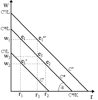
Now, for a given technique K/L and a given cost level C, we can derive a factor-price curve which gives the different combinations of w and r which, at a given K/L, yield the same cost C. [Note: when dealing with applications to economy-wide equilibrium, economists normally assume constant returns to scale so that they can write Y = rK + wL by Euler's theorem, and then proceed to trace out factor price curves and frontiers from there; in that case, the factor price frontier can be conceived as the dual of the production function and an economy-wide equilibrium locus. We shall refrain from that maneouvre here, and concentrate solely on cost; albeit see our discussion of the Cambridge Capital Controversy.] In Figure 8.7, we have a series of factor-price curves all for a given capital-labor ratio k = K/L, thus, they all have slope k = K/L. Notice that the vertical intercept of the factor-price curve denotes a particular cost level, C/L (the horizontal intercept is C/K). Thus, as C¢ < C* < C¢¢ , then factor price curve C¢ represents lower costs than C* which in turn represents lower costs than C¢¢ .
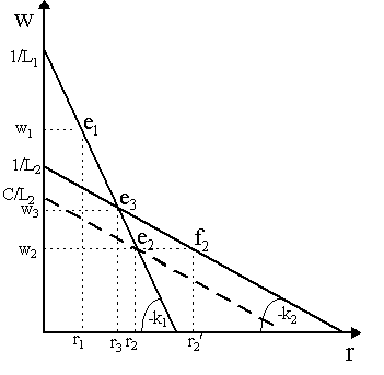
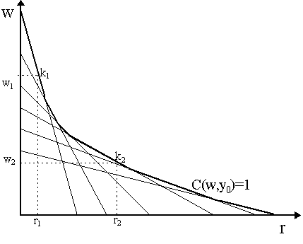
To understand the meaning of a factor price curve, it is useful to imagine that we have a Leontief production technology - thus, constant factor proportions, which is captured here by k. Suppose w = w1 and r = r1, so that we are at e1 in Figure 8.7. At these factor prices, total costs are C*. Suppose now w decreases to w2 so that we have factor price combination (w2, r1), shown in Figure 8.7 by e1¢ . As nothing else changes, costs will fall, thus we move to the lower factor-price curve, C¢ . However, in order to return to the same cost level C*, we therefore need to raise r to r2. Thus, e1 = (r1, w1) and e2 = (r2, w2) represent the same amount of total costs. Similarly, if we start from e1 and raise r to r3, then total costs will rise to C¢ ¢ . Thus, lowering w to w3, we will return to the same cost level C*. Thus, e1 = (r1, w1) and e2 = (r3, w3) represent the same total costs C*. More straightforwardly, note that everywhere on a given factor price curve, we have wL + rK = C*, thus as C*, K and L are given, then if w goes down, r must go up to keep costs at C*. In Figure 8.8 we have drawn two different factor curves corresponding to two different capital-labor ratios, k1 = K1/L1 and k2 = K2/L2 and the same cost level, which we normalize to C = 1 (ignore the dashed line for the moment). Thus, factor-price curve associated with k1 has slope - k1, vertical intercept 1/L1 and horizontal intercept 1/K1 whereas the other factor price curve is associated with k2 has slope -k2, vertical intercept 1/L2 and horizontal intercept 1/K2. Notice that the factor price curve k1 is steeper than k2, thus we know that k1 > k2, i.e. the steeper the factor price curve, the more capital-intensive (less labor-intensive) the corresponding k is.
Reading Figure 8.8 is a little tricky due to the normalization to unit costs, Nonetheless, consider the capital-intensive technique k1. The formula for this factor price curve is:
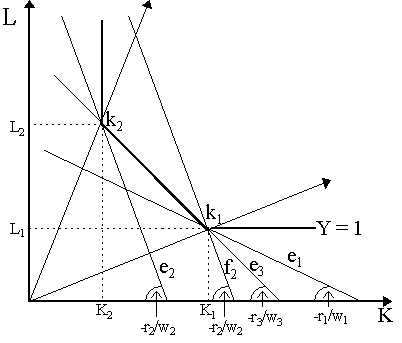
Thus, for a given r (or given w), we can find the corresponding wage w (or corresponding r) that yields total costs 1 at that given technique k1. Consider wage w1; the corresponding rental rate on capital is r1, shown at e1. Similarly, at wage w2, the corresponding rental rate on capital that yields unit costs for technique k1 is r2, shown by point e2. In contrast, notice that the factor price curve for the labor-intensive technique k2 is governed by w = 1/L2 - (K2/L2)r. Following the same logic, then when wage is w2, the rental rate on capital that yields unit costs for technique k2 is r2¢ , as shown by point f2. Notice that at w3, the corresponding rental rates for both techniques is r3, as shown by point e3. The usefulness of the factor price curves is that we can trace the cost-minimizing choice of technique by the "rule of the outermost". Specifically, at any given real wage w, we can detect what the chosen cost-minimizing technique is by choosing the technique that yields the highest r. Thus, in Figure 8.7, when w = w1, the cost-minimizing choice of technique is k1. When w = w3, the cost-minimizing choice of technique is both k1 and k2 (we are indifferent between techniques). Finally, when w = w2, the cost-minimizing choice of technique is k2 and not k1. The "rule of the outermost" may not seem to make much intuitive sense in this last case: at w = w2, the r corresponding to k1 is r2 while the r corresponding to k2 is r2¢ . But if r2¢ > r2, don't we have greater costs using technique k2 than technique k1? No. Total costs, as we noted, are the same on both factor price curves k1 and k2 as we have normalized costs to 1. In other words, costs to using technique k1 at factor prices r2/w2 are the same as the costs to using technique k2 at factor prices r2¢ /w2. However, it is precisely because total costs are the same on both factor price curves that we can say that k2 is a cost-minimizing choice of technique when w = w2. To see why, note that if we decided to use technique k2 at factor prices r2/w2, i.e. if we were forced to stay at point e2, then we would be off the factor price curve k2. In other words, we would not be incurring unit costs at e2 but rather less than unit costs. We can see this via the parallel dashed line passing through e2 in Figure 8.8, which represents technique k2 when forced to use prices r2/w2. Notice that the costs represented by this dashed curve are lower than unit costs (compare the intercepts, C/L2 for the dashed line and 1/L2 for the unit factor price curve for technique k2; obviously, C < 1). In other words, using technique k2 at factor prices r2/w2 yields lower costs (i.e. C2) than using technique k1 at factor prices r2/w2 (which yields unit costs). The "rule of the outermost", therefore, merely captures the idea of cost-minimization, while keeping total costs normalized to 1. The meaning of Figure 8.8 can best be gathered by reading it in conjunction with the more familiar Figure 8.9, where we have depicted the activity analysis unit isoquant when we only have two techniques, k1 and k2. If relative factor prices are low at r1/w1, we obtain a whole series of isocost curves with slope - r1/w1. Notice that minimizing costs in the isoquant space, we would choose the capital-intensive technique k1, yielding isocost curve C1. If factor prices increased to r2/w2 and we stayed on the same technique k1, the isocost curve would swivel to C2 in Figure 8.9. But this is not the cost-minimizing thing to do. Facing prices r2/w2, costs would be minimized if we moved to the labor-intensive technique k2 and corresponding isocost curve C2¢ . Finally, notice that if factor prices are r3/w3, the isocost curves are parallel to the isoquant segment between k1 and k2. Cost-minimization, in this case, leaves us with an indeterminate input choice: k1, k2 or any convex combination of these would all be cost-minimizing at those factor prices. Notice that point e3 in Figure 8.8 is often called a switchpoint as it denotes the the factor prices at which we move from one technique to another. Notice that it is quite sensitive: a slight rise in w leads to a complete switch to k1, a slight fall in w leads to a complete switch to k2.
The cost-minimization exercise in isoquant-isocost space in Figure 8.9 is precisely captured by the "rule of the outermost" with factor-price curves in Figure 8.8. When wages are w1, the rule of the outermost tells us the optimal technique is k1, thus k1 is chosen. As wages decline to w2, the rule of the outermost tells us we choose k2. This is effectively equivalent to a unit-cost-normalized version of the move from r1/w1 to r2/w2 in the non-normalized case in Figure 8.9. Notice also that when the wage is w3, the rule of the outermost tells us that we are indifferent between k1 and k2: this corresponds to the indeterminacy in r3/w3 in Figure 8.9. Thus, although our normalizations make them seem different, choosing cost-minimizing isocost curves in the capital-labor space as in Figure 8.9 yields exactly the same information about cost-minimizing input choices as when we follow the "rule of the outermost" in factor price space. The information in both diagrams is effectively the same. Adding more techniques in capital-labor space translates into adding more activity rays to the point where we might get a smooth isoquant. Similarly, in factor price space, adding more techniques, would add more factor-price curves. In the limit, as the number of activities increases to infinity, we would be able to trace a factor price frontier as the envelope of the factor price curves. This is shown in Figure 8.10 by the thick line C(w, y0) = 1. Notice that the factor price frontier follows the "rule of the outermost" for all the factor price curves. [the "factor price frontier" is Samuelson's (1962) term; Hicks (1965: p.150) calls it the "wage frontier"; Neo-Ricardians (e.g. Kurz and Salvadori, 1995: p.50) tend to call it the "wage-profit frontier".]
The reason for labelling the factor price frontier as C(w, y0) = 1 is precisely because it represents the combinations of factor prices that, by cost-minimization, yield unit costs. In fact, it should be detected that the the factor price frontier in Figure 8.10 represents a unit contour of the cost function for a given output level y0. This is intuitive. We previously demonstrated that the cost function C(w, y) was concave with respect to factor prices, thus, in effect, the cost function is a "hill" over factor prices. We know that the upper contour set of a concave function is convex. This is precisely what we have here: the factor price frontier is merely the unit contour line of the "cost hill" and it is, indeed, convex. Computing the slope of the factor price frontier is obtained by differentiating the cost function at a given output level, C(w, y0), with respect to factor prices. Using the implicit function rule:
But, by Shephard's Lemma, we know that ¶ C(w, y0)/¶ w = L and ¶ C(w, y0)/¶ r = K, thus ¶ w/¶ r = -K/L. Thus, at any particular factor price combination in Figure 8.10, the corresponding slope of the factor price frontier is the (negative of) the factor input ratio K/L that minimizes costs at those factor prices. This, of course, is precisely the "rule of the outermost" that is traced by the factor price frontier. Notice two other interesting results. The first (obvious) one, as we have already seen, is that if w falls and r rises (i.e. r/w rises), then the cost-minimizing choice of inputs will be more labor-intensive, e.g. we move from capital-intensive k1 to labor-intensive k2 in Figure 8.10. This is the standard result of the derived demand for factors we obtained earlier: the demand for a factor falls when its price rises. Notice a second implication. A ray from the origin in factor price space will have slope w/r, while the wage-profit frontier will have slope K/L. Consequently, we can measure the curvature of the factor price frontier by the formula:
which one will recognize immediately, as w/r = ¦ L/¦ K by cost-minimization, to be the inverse of the elasticity of substitution, s , i.e. h = 1/s . Thus, when the elasticity of substitution is very low, e.g. s = 0 as in the Leontief case, then h = ¥ , i.e. the factor-price frontier is completely linear. But we have already seen this: as noted earlier, when there is a single technique, as in Leontief, the factor price frontier collapses to a single factor price curve which is, of course, linear. The converse applies: factor price frontiers take on an L-shape when s = ¥ , i.e. perfect substitution among factors. Thus, the more curved isoquants are, the less curved the factor price frontier is.
|
All rights reserved, Gonçalo L. Fonseca

