(1) Introduction
(2) Commodities and Preferences
(3) Utility Functions
(4) Budget Constraints
(5) Demand
(6) Properties of Demand
(7) Generalized Law of Demand

Selected References

Back

(1) Introduction

The utility-based theory of consumer demand was one of the cornersones of Neoclassical theory. The Marginalist Revolutionaries, William Stanley Jevons (1871), Carl Menger (1871) and Léon Walras (1874) all appealed to the notion of utility-based theory of price, although only Walras bothered to derive demand from utility explicitly.

The basis for the theory was much older. Augustin Cournot (1838) was the first to introduce demand as a function of its own price, although it was Walras (1874) who made it a function of all prices. The concept of utility and diminishing marginal utility was already in the work of Daniel Bernoulli (1738). The notion of utility, of course, was made famous by Jeremy Bentham (1789) and many proto-marginalist economists - such as Auguste Walras (1831),  W.F. Lloyd (1934),  Jules Dupuit (1844) and Heinrich Gossen (1854) attempted to apply it to economic theory. The indifference curve was introduced by Francis Y. Edgeworth (1881) and the irrelevance of a cardinal scale established independently by Irving Fisher (1892) and Vilfredo Pareto (1896). It was Pareto (1896, 1906) who gave great relevance to the notion of "preference" and "choice" rather than utility functions, as the foundation of demand.

The Paretians, notably Vilfredo Pareto (1906), W.E. Johnson (1913), Eugen Slutsky (1915), John Hicks and R.G.D. Allen (1934), John Hicks (1939) and Paul Samuelson (1947) provided increasingly more general derivations of demand from utility-maximization and described the properties of demand functions fully.

The mathematical axiomatization of the theory of choice was initiated by Ragnar Frisch (1926) and followed up by Oskar Lange (1934), Franz Alt (1936), S. Eilenberg (1941), Hermann Wold (1943-4), with a great impetus given by John von Neumann and Oskar Morgenstern (1944). Giovanni Antonelli (1886) was the first to pose the "integrability" problem of deriving preferences from observed demand. This was followed up by Nicholas Georgescu-Roegen (1936) and Paul Samuelson (1938, 1947).

For more details on the history of demand theory consult Stigler (1950), Katzner (1970) or our brief history of the phases of the Marginalist Revolution.  The following presentation adopts much of the Neo-Walrasian presentation in Gérard Debreu (1959)

(2) Commodities and Preferences

The "commodity set" is often defined as X Ì Rⁿ, thus there are n commodities. We shall take X = Rⁿ and thus X is convex (complete divisibility of commodities). For infinite-dimensional commodity sets, see our discussion elsewhere.

An element x Î X is a "commodity bundle" or "net consumption vector". If a particular entry is positive (x_i ³ 0), then that good is a consumable good whereas if that entry is negative (x_i £ 0) then it is a factor.

Let H be the set of agents and, abusively of notation, let #H = H (i.e. we have H agents). An agent can effectively be defined as the triplet (C^h, ³_h, e^h) - where C^h is his/her consumption set, ³ _h are his/her preferences and e^h his/her endowment.

The consumption set, C^h, is a subset of the commodity space, X and denotes the bundles of commodities that are relevant to agent h. The main point about C^h is that it is bounded from below by agent h (i.e. she won’t even consider certain bundles, e.g. those that require that she work more than 24 hours a day or consumes less than some survivable minimum). It is assumed that C^h is closed, convex, connected and bounded from below.

The hth consumer’s preferences, ³ _h, are a complete preordering over bundles in the consumption set. Specifically, we define the binary relation ³ _h Ì C^h ´ C^h as indicating "preferred to or equivalent", then (x, y) Î ³ _h or, equivalently, x ³ _h y denotes that bundle x is preferred to or equivalent to bundle y by consumer h. On the basis of this, we can define the following two additional binary relations:

>_h - "strictly preferred to" - where x >_h y if  "not x  £ _h y".

~_h - "equivalent to"/"indifferent to" - where x ~_h y if "x ³ _h y and y ³ _h x".

We can also define the following two sets relative to a bundle x:

Upper contour set: R^h(x) = {y Î C^h ½ y ³ _h x} - the set of points preferred to or equivalent to x.

Strict upper contour set: P^h(x) = {y Î C^h ½ y >_h x} - set of points strictly preferred to x.

Indifference set: I^h(x) = {y Î C^h ½ y ~_h x} - set of points equivalent to x.

The following six axioms are commonly assumed on preferences:

Axioms of Preferences

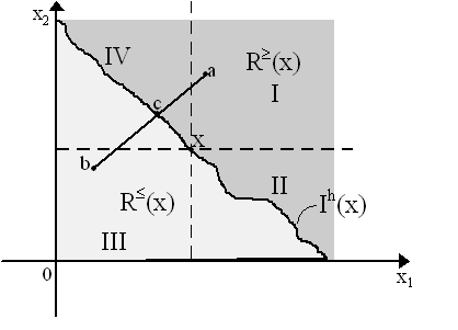
Axiom (2) is in fact superfluous as it is implied by combining (1) and (3).

Figure 1 - Axioms of Preference

If we imposed a strict monotonicity version of Axiom 4 and transitivity (Axiom 3), we know that not more than one point on that line will be indifferent to x. Why? for any two points c and d on that line, then either d is greater than c or c is greater than d. Suppose the former, in which case strict monotonicity implies d >_h c. Let us nonetheless suppose that c ~_h x and d ~_h x. It is elementary to see that, by transitivity (Axiom 4), c ~_h d, which contradicts strict monotonicty. Thus, c is the unique point of indifference on the chord (a, b).

We can construct more lines of this type connecting bundles in quadrants I and III and thus derive a whole array of indifference points akin to point c. There will thus be a set of points in C^h which are "indifferent" to x, denoted in Figure 1 by the wavy line I^h(x), the indifference set.

Finally, by Axiom 6, we are stating that the set R^h(x) is convex - which implies, in turn, that the indifference set is not the wavy line shown in Figure 1, but rather is convex to the origin. Thus, Axioms (1)-(6) enables us to construct the familiar convex-shaped indifference curve relative to point x. Doing this for any x Î C^h, we obtain the entire indifference map so familiar in microeconomics - with transitivity (Axiom 3) helping us guarantee that these do not intersect.

(2) Utility Functions

Utility is defined as a real-valued, continuous, order-preserving function U^h: C^h ® R. We say this utility index "represents" preferences if U^h(x) ³ U^h(y) whenever x ³ _h y. Axioms (1)-(4) are required to prove the existence of a utility function to represent preferences. Proof of existence of a utility function on the basis of the first four axioms was first set forth by Debreu (1954).

Theorem: (Representation) If preferences ³ _h satisfy Axioms (1)-(4) and C^h is a connected topological space having a denumerable dense subset, then there is a real-valued, continuous function U^h: C^h ® R such that for any x, y Î C^h, we have U^h(x) ³ U^h(y) whenever x ³ _h y.

We could go on to prove continuous representability, but shall omit that and refer to the far more general proofs elsewhere, e.g. Debreu (1954, 1959: Th. 4.6.1.), Rader (1963) or Katzner (1970).

That any increasing transformation of U^h will not affect representability of preferences is easy to show. Let U^h: C^h ® R represent preferences, then let T be an increasing transformation of U^h. Thus, by definition, if U^h(x) ³ U^h(y) then T(U^h(x)) ³ T(U^h(y)) for any x, y. Combining, then (T·U^h)(x) ³ (T·U^h)(x). Thus, when x ³ _h y Þ U^h(x) ³ U^h(y) Þ (T·U^h)(x) ³ (T·U^h)(x) thus T·U^h: C^h ® R also represents preferences.

If convexity (Axiom 6) is added, then the utility function U^h will be quasi-concave and the sets P^h(x) and R^h(x) will be convex. If we impose strict convexity, then equivalently we have strict quasi-concavity of utility and strict convexity of the upper contour sets. Proofs of this are elementary:

Theorem: (Quasi-Concavity of Utility Function) If U^h: C^h ® R is a utility function representing preferences ³_h, then if ³ _h is convex, then U^h is quasi-concave.

Proof: If ³ _h is convex, then given any x, y Î C^h where y ³ _h x then l y + (1-l )x ³ _h x. ). Thus, by representability, this translates to the following: U^h(y) ³ U^h(x) implies U^h(l y + (1-l )x) ³ U^h(x). This is already the definition of quasi-concavity of U^h. To be sure, define the upper contour set R(x) = {z Î Rⁿ | U^h(z) ³ U^h(x)}. Thus, if x, y Î R(x), then convexity of preferences implies l x + (1-l )y Î R(x). Thus, R(x) is convex. Consequently, U^h is quasi-concave.§

(3) Budget Constraints

A budget set is defined as B^h: P ´ Rⁿ ® Cⁿ, i.e. a budget set is a correspondence from the price space (P Ì Rⁿ) and the commodity set (Rⁿ) to the consumption set (C^h). From the former two, we take the given prices p Î P and the endowent bundle, e^h, of agent h. Thus, we can define the budget set as:

B^h(p, e^h) = {x Î C^h ½ px £ pe^h , p Î P}

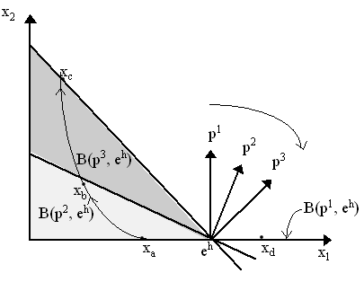
i.e. the set of bundles in the consumption set that are affordable to agent h.

The budget set correspondence is upper semicontinuous but not necessarily lower semicontinuous with respect to prices. To see this, consider Figure 2. Notice that as p changes from p¹ to p² to p³, the budget constraint changes from B(p¹, e^h) to B(p³, e^h).to B(p³, e^h). To verify whether B(·, e^h) is upper semicontinuous, then, heuristically, all we have to do is take a convergent sequence pⁿ ® p, construct the budget constraint for each price, B(pⁿ, e^h), and then find a convergent sequence of bundles x_n ® x such that each bundle is within each constraint (x_n Î B(pⁿ, e^h)). Then, the budget set correspondence would be upper semicontinuous if the limiting bundle x of every sequence of bundles drawn out this way is itself within the limiting budget constraint, i.e. x Î B(p, e^h).

This is seen in the Figure 2: suppose p ® p³, then as we move from p¹ to p² to p³, we can take a sequence stemming from x_a to x_b to x_c with, obviously, limiting bundle x_c Î B(p³, e^h). Conversely, suppose p ® p¹, then we can go backwards or, more simply, we can start at point such as x_a Î B(p³, e^h) and as we move from p³ to p² to p¹, we continue to stay at point x_a. Thus, the limiting point x_a Î B(p¹, e^h). We can do this for any sequence drawn, thus the budget set is upper semicontinuous.

However, the budget set is not lower semicontinuous. To see this, consider the following. Heuristically, lower semicontinuity implies that we choose an endpoint first and then find a sequence of bundles in the sequence of budget sets which converge to it. However, in Figure 2, if we consider sequence p ® p¹ and choose bundle x_{d Î} B(p¹, e^h) as our endpoint, then it is obvious that in the sequence of buget constraints as p ® p¹, there is no sequence of bundles x_n ® x_d. Thus, the budget set is not lower semicontinuous.

In order to obtain lower semicontinuity, we need to rule out cases such as in the Figure 2. One way would be to impose the "locally cheaper point property": pe_i^h ¹ min px_i, or, equivalently, there is an x Î Bⁿ(p, e^h) such that px < pe_h. Intuitively, this implies that there is always a bundle in the budget set that is "cheaper" (however slightly) than the value of the endowment. Notice that an alternative way of ensuring lower semicontinuity, i.e. requiring positivity of all prices, would be far too strict for we would be ruling out free goods a priori. Thus, assuming the "cheaper point property" is a bit more reasonable from an economic viewpoint.

Finally, we should note that the budget set is non-empty (because of endowment), convex (obvious), closed (because of upper semicontinuity) and bounded above (by the price line). However, it is not compact because there is not necessarily a lower bound as well. However, because we have assumed earlier that the consumption set C^h itself has a lower bound, then the intersection B^h(p, e^h) Ç C^h is closed and bounded and thus, by Heine-Borel, compact. Perhaps abusively of notation, we shall assume henceforth that B^h(p, e^h) = B^h(p, e^h) Ç C^h - thus when claiming "the budget set" we mean only the economically-relevant portion of it. In other words, when we construct our B^h(p, e^h), we shall assumed it is for bundles drawn out of the consumption set C^h, as opposed to the commodity set, thus we are already making B^h(p, e^h) compact.

 (4) Demand

An agent’s demand is defined as a correspondence f^h : P´ Rⁿ ® C^h - or a set-valued mapping f^h (p, e^h) from price-endowment pairs to bundles in the consumption space. These arise from the maximization of utility functions subject to the budget set. Thus, we can define the following:

y^h (p, e^h) = max U^h(x) s.t. x Î B^h(p, e^h)

f^h (p, e^h) = argmax U^h(x) s.t. x Î B^h(p, e^h)

where the first function (the "maximized utility") is a real-valued functon y ^h: P ´ Rⁿ ® R which maps from price-endowment pairs to utility. The function y ^h(p, e^h) is better known as the "indirect utility function". The argmax of the indirect utility function (i.e. the "arguments" that maximize indirect utility) is, of course, the (Marshallian) demand correspondence, f^h (p, e^h).

The first thing we need to establish is the existence of demand. This is easily done by appealing to the Weierstrass Theorem: as U^h is a continuous, real-valued function over a non-empty, compact set B^h(p, e^h), then a maximum exists, i.e. y^h(p, e^h) exists and, consequently, so does demand f^h(p, e^h). Now, because U^h is a continuous function and B^h(p, e^h) is both an upper and lower semicontinuous correspondence, then by Berge’s Theorem we also know that y ^h(.) is a continuous function and that demand f^h(.) is an upper semicontinuous correspondence.

Alternatively, we could have considered the dual case of expenditure minimization, first suggested by Paul Samuelson (1947) and set down finally by Lionel McKenzie (1957) by defining the following two terms:

E^h(p, U_o^h) = min px s.t. x Î {y Î C^h ½ U^h(y) ³ U₀^h }

h^h(p, U_o^h) = argmin px s.t. x Î {y Î C^h ½ U^h(y) ³ U₀^h }

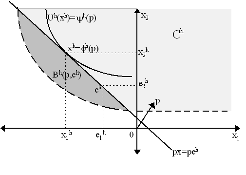
where the first term E^h(p, U₀^h) is the expenditure function (or cost function) and the second term h^h(p, U₀^h) is the compensated or Hicksian demand correspondence. It is easy to show that E^h(p, U_o^h) is continuous and that {y Î C^h ½ U^h(y) ³ U₀^h }is closed and bounded below, thus by a weaker form of Weierstrass Theorem, there is necessarily a minimum, i.e. a cost-minimizing bundle h^h(p, U_o^h), or a Hicksian demand. Furthermore, {y Î C^h ½ U^h(y) ³ U₀^h } is constant, thus it is both upper semi-continuous and lower semicontinuous. Consequently, by Berge’s theorem, the expenditure function is continuous and the Hicksian demand function upper semicontinuous.

The two-dimensional Figure 3 depicts succinctly the household's utility-maximization decision where x₁ is a factor (and thus negative in the net consumption vector, x) while x₂ is a consumable good (and thus positive in the net consumption vector). We can think of them as labor and bread, respectively. The consumption space is denoted C^h and corresponds to the lightly shaded region. Note that the dashed line forms the lower bound to the consumption space - agents will not consider bundles below this amount. The consumer's endowment is denoted e^h and note that it is within the consumption space C^h, thus it is "survivable", i.e. if agents decide not to trade, they can at least live on their endowment. A given set of prices, p, defines a hyperplane {y Î Rⁿ | px = pe^h}which passes through the endowment point and below that (and above the lower bound of C^h) we obtain the budget set, B^h(p, e^h).

Agents' preferences are represented by a utility function U^h. This is captured by indifference curves which ascend in Figure 3 in a northeasterly direction, representing the fact that the agent prefers to consume more of good 2 (the consumption good) and supply less of the amount of good 1 (the factor). Maximizing utility subject to the budget set, agent h will choose f ^h(p, e^h) = x^h = [x₁^h, x₂^h] as the maximal element - by which we mean she will demand x₂^h of good 2 and supply x₁^h of factor 1. The indirect utility amount y ^h(p, e^h) = U^h(x^h) represents the utility gained by the consumer from her demand, x^h.

The expenditure minimization exercise is analogous and achieves the same solution, albeit here we take U(x^h) as given and choose minimize cost px^h at a given price, i.e. choose a bundle x^h by shifting the hyperplane px towards the origin. The cost-minimizing bundle, h^h(p, U_o^h) ought to be the same as the utility-maximizing bundle f ^h(p, e^h) if the prices facing the consumer are the same in both cases and the utility constraint of the cost-minimizing exercise is the same as the indirect utility function of the utility-maximizing exercise (i.e. U_o^h = y ^h(p, e^h)) and/or equivalently, the sale amount of the endowment in the utility-maximizing exercise is the same as the expenditure achieved in the expenditure-minimizing exercise (i.e. pe^h = E^h(p, U_o^h)). This relationship between utility-maximization and expenditure-minimization is referred as the consumer duality theorem and was first laid out in full by Lionel McKenzie (1957).

(5) Properties of Demand

Most of the properties denoted here should be familiar from standard microeconomics. We shall work here with cost functions E^h(p, U_o^h) and Hicksian demand, h^h(p, U_o^h). For simplicity, we shall suppress household superscript h as we are doing this for one household.

Theorem: The cost function E(p, U_o) is homogeneous of degree one in prices, p.

Proof: Recall that E(p, U_o) = min px s.t. x Î {y Î C^h ½ U(y) ³ U₀ } which we can rewrite as E(p, U_o) = min _{{xÎ C: U(x) ³ Uo}} å _i p_ix_i. Thus, for any real numbert a > 0, we have it that E(a p, U_o) = min _{{xÎ C: U(x) ³ Uo}} å _i a p_ix_i. However as a is a constant scalar then E(a p, U_o) = a [min _{{xÎ C: U(x) ³ Uo}} å _i p_ix_i] or E(a p, U_o} = a E(p, U_o) by definition.§

Theorem: The cost function E(·, U_o) is concave in prices.

l E(p₁, U_o) + (1-l )E(p₂, U_o) £ E(l p₁ + (1-l )p₂, U_o)

which is the definition of concavity. Thus E(p, U_o) is concave in prices.§

Theorem: (Shephard's Lemma) If E(p, U_o) is a differentiable function, then dE/dp_i = h(p, U_o) for any i

Proof: Recall from our definitions that E(p, U_o) = min _{{xÎ C: U(x) ³ Uo{} å _i p_ix_i. Letting h_i(p, U_o) be the Hicksian demand for the ith good (i.e. h_i(p, U_o) is the ith element of the vector h(p, U₀)), then substituting that in, at the optimum:

E(p, U_o) = å _i p_ih_i(p, U_o)

h_i(p, U_o) is derived from the cost-minimization exercise. Assuming differentiability, then differentiating with respect to p_i:

¶ E(p, U_o)/¶ p_i = h_i(p, U_o) + å _j p_j (¶ h_j/¶ p_i)

But using the envelope theorem, we know that å _j p_j(¶ h_j/¶ p_i) = 0 as h_j(p, U_o) is already the optimal choice, so then:

¶ E(p, U_o)/¶ p_i = h_i(p, U_o)

which is Shepherd’s Lemma.§

Theorem: (Negative Own-Substitution Effects) For any commodity i, ¶ h_i/¶ p_i £ 0

Proof: Assuming the cost function is twice differentiable, then from Shephard’s Lemma, ¶ E(p, U_o)/¶ p_i = h_i(p, U₀). So, differentiating again with respect to p_i, ¶ ²E(p, U_o)/¶ p_i² = ¶ h_i(p, u_o)/¶ p_i. But as we also showed that E(p, U_o) was concave with respect to p_i, then ¶ ²E(p, U_o)/¶ p_i² = ¶ h_i(p, U_o)/¶ p_i £ 0.§

Let us now turn to defining substitute and complementary goods.

Substitutes: Goods i ¹ j are considered to be substitutes if ¶ h_i(p, U_o)/dp_j ³ 0 and ¶ h_j(p, U₀)/dp_i ³ 0.

Complements: Goods i ¹ j are considered to be complements if ¶ h_i(p, U_o)/dp_j £ 0 and ¶ h_j(p, U₀)/dp_i £ 0.

Theorem: In a two-commodity world, both commodities will necessarily be substitutes for each other.

Proof: Let us consider the two good case, x₁ = h₁(p, U_o) and x₂ = h₂(p, U₀). By Shephard’s Lemma and assuming twice differentiabile cost functions, then:

¶ ²E(p, U_o)/¶ p_1¶ p₂ = ¶ h₁(p, U_o)/¶ p₂

and

or:

[¶ h₁(p, U_o)/¶ p₁]p₁ + [¶ h₂(p, U_o)/¶ p₁]p₂ = 0

Similarly by homogeneity:

[¶ ²E(p, U_o)/¶ p₂²]p₂ + [¶ ²E(p, U_o)/¶ p₁ ¶p₂]p₁ = 0

or

[¶ h₂(p, U_o)/¶ p₂]p₂ + [¶ h₁(p, U_o)/¶ p₂]p₁ = 0

so, recognizing that p₁ ³ 0 and p₂ ³ 0 (by definition of price) and recalling by the concavity of expenditure functions that dh₁(p, U_o)/dp₁ £ 0 and dh₂(p, U_o)/dp₂ £ 0, then it must be true that if assuming p₁ and p₂ are non-zero, that:

¶ h₁(p, U_o)/¶ p₂ = - [¶ h₂(p, U_o)/¶ p₂]p₂/p₁ ³ 0

¶ h₂(p, U_o)/¶ p₁ = - [¶ h₁(p, U_o)/¶ p₁]p₁/p₂ ³ 0

i.e. goods 1 and 2 are substitutes. Thus, in a two commodity world, commodities must be substitutes to each other.§

Theorem: (Symmetry of Cross-Effects) For any two commodities 1 and 2, ¶ h₁(p, U_o)/¶ p₂ = ¶ h₂(p, U_o)/¶ p₁, i.e. cross effects are symmetric.

Proof: We have already shown that ¶ ²E(p, U_o)/¶ p_1¶ p₂ = ¶ h₁(p, U_o)/¶ p₂ and ¶ ²E(p, U_o)/¶ p_2¶ p₁ = ¶ h₂(p, U_o)/¶ p₁. By Young’s Theorem, ¶ ²E(p, U_o)/¶ p_1¶ p₂ = ¶ ²E(p, U_o)/¶ p_2¶ p₁, thus ¶ h₁(p, U_o)/¶ p₂ = ¶ h₂(p, U_o)/¶ p₁.§

Note the interesting implication of symmetry: economically, this means that increasing the price of good 1 will increase the demand for good 2 by the same proportion that increasing the price of good 2 will increase the demand for good 1. This is interesting in that it may not seem that intuitive, but it is not altogether surprising.

Theorem: For any l Î Rⁿ, å_i å_j l_i l_j[¶ h_i(p, U₀)/¶ p_j] £ 0.

Proof: As the cost function E(p, U_o) is concave, then we can define the n x n Hessian matrix:

	é	¶2E(.)/¶p12	......¶ 2E(.)/¶ pi ¶ p1	.....¶ 2E(.)/¶ pn ¶ p1	ù
	ê	:	:	:	ú
H =	ê	¶2E(.)/¶p1 ¶ p	......¶ 2E(.)/¶ pi2	......¶ 2E(.)/¶ pn ¶ pi	ú
	ê	:	:	:	ú
	ë	¶ 2E(.)/¶p1 ¶ pn	......¶ 2E(.)/¶ pi ¶ pn	......¶ 2E(.)/ ¶ pn2	û

where the concavity of E(p, U_o) implies that the Hessian matrix, H, is negative semi-definite. By this we mean that pre-multiplying and post-multiplying by any n-dimensional vector l ‘ = [l _1, l ₂, ...., l _n], then l ‘Hl £ 0, or:

l ‘Hl =  å_i å_j l_i l_j [¶ ²E(p, U_o)/¶ p_i ¶ p_j] £ 0

but by the corollary to Shephard’s Lemma, we know that [¶ ²E(p, U_o)/¶ p_i ¶ p_j] = ¶ h_i(p, U₀)/¶ p_j. Thus:

l ‘Hl = å_i å_j l_i l_j[¶ h_i(p, U₀)/¶ p_j] £ 0

which is what we sought.§

(6) Generalized Law of Demand

Paul Samuelson’s (1938, 1947) theory of revealed preference attempted to reduce many of the axioms of consumer behavior to a single inductive axiom: the weak axiom of revealed preference (WARP) which essentially argued that an agent’s preference of x over y is "revealed" if he chooses x when y is available and when he chooses y, x is more expensive, i.e. if x is chosen at p_x (which implies, in our terms, x Î h(p_x, U_o)) and y is chosen at p_y (which implies y Î h(p_y, U₀)) then WARP claims x is revealed preferred to y if p_xx ³ p_xy implies p_y x > p_yy. The question was posed at least since Georgescu-Roegen (1936): can utility functions or preferences be constructed by an inductive law of demand? Addressing this "integrability" problem was the original purpose of WARP and for more on this, see Uzawa's (1960) classical piece, or Katzner (1970) for an excellent review.

For our puproses, we hope merely to show that a version of WARP can be derived from the expenditure-minimization exercise. If indeed, x Î h(p_x, U_o)) and y Î h(p_y, U₀) then we know by the definition of h(·), that U(x), U(y) ³ U₀, so both x and y are feasible under both prices. Then by definition of compensated demand p_xx £ p_xy and p_yy £ p_yx which is analagous to WARP. Rearranging these inequalities, p_x (x - y) £ 0 and p_y(x - y) ³ 0 so that combining pointwise, p_x (x - y) £ p_y(x - y), or:

(p_x - p_y)(x - y) £ 0

which is a "generalized law of demand". How? Suppose p_x = p_y + e r_i where e > 0 is a scalar and r_i = (0, 0, ...., 1, ....0, 0), i.e. an n-dimensional vector with a 1 in the ith position and 0 elsewhere, then this law can be rewritten as:

(p_y + e r_i - p_y)(x - y) £ 0

or:

e r_i(x - y) £ 0

or:

e (x_i - y_i) £ 0

where x_i and y_i are the ith elements of the vectors x and y respectively. From this we see (as e can be made abitrarily small) that x_i £ y_i. In other words, if we raise the price of good i by a unit, then the demand for good i will fall (or rather not increase) if the ith good is an output (i.e. x_i, y_i ³ 0). If the ith good is an input (i.e. x_i, y_i £ 0), then we see that this result implies |x_i| ³ |y_i|, i.e. the supply (by the consumer) of input i increases (or does not fall) as its price rises.

The strength of this generalized law of demand (and supply) is that we do not need to go much beyond the conditions of the Weierstrass Theorem, i.e. for a given U_o, we must presume that the points x Î h(p_x, U₀) and y Î h(p_y, U₀) exist and are well-defined - which requires, by Weierstrass, the continuity of the utility function U and that C^h is non-empty and compact set. However, we do not need to say anything about differentiability or twice-differentiability of the cost function E(p, U_o) as we did earlier. However, the generalized law may be less precise quantitatively.

Selected References

Gérard Debreu (1954) "Representation of a Preference Ordering by a Numerical Function", in Thrall et al., editors, Decision Processes. New York: Wiley.

Gérard Debreu (1959) Theory of Value: An axiomatic analysis of economic equilibrium. New York: Wiley.

Nicholas Georgescu-Roegen (1936) "The Pure Theory of Consumer's Behavior", 1936, Quarterly Journal of Economics, Vol. 50, p.545-93.

Donald W. Katzner (1970) Static Demand Theory. New York: Macmillan.

Lionel W. McKenzie (1957) "Demand Theory without a Utility Index", Review of Economic Studies, Vol. 24, p.185-9.

Paul A. Samuelson (1947) Foundations of Economic Analysis. 1983 edition. Cambridge, Mass: Harvard University Press.

George J. Stigler (1950) "The Development of Utility Theory, I & II", Journal of Political Economy, Vol. 58, (4) p.307-27, (5), p.373-96.

Hirofumi Uzawa (1960) "Preferences and Rational Choice in the Theroy of Consumption", in K.J. Arrow, S. Karlin, P. Suppes, editors, Mathematical Methods in the Social Sciences. Stanford: Stanford University Press.

Top

Back