|
____________________________________________________________________________
____________________________________________________________________________ (1) The Cass-Koopmans
Model (1) The Cass-Koopmans Model Although Frank Ramsey presented the original model of optimal growth back in 1928, the "modern" version which connected it more deeply to Solow-Swan Neoclassical growth theory was introduced independently by David Cass (1965), Tjalling C. Koopmans (1965), Edmond Malinvaud (1965) and Paul A. Samuelson (1965). The main impetus for this resurrection was the work of T.N. Srinivasan (1964) and Hirofumi Uzawa (1964) in two-sector growth models, where they maximized the integral of a consumption path (not utility) in order to pin down a solution. Notable contributions to optimal growth model in its early stages include James A. Mirrlees (1967), Karl Shell (1967) and Kenneth J. Arrow and Mordecai Kurz (1970). Despite the plethora of economists involved in its early development, the optimal growth model presented here has become known simply as the "Ramsey model" or the "Ramsey-Cass-Koopmans" model. To differentiate Ramsey's original model from this one, we shall call it simply the "Cass-Koopmans" optimal growth model. (a) Set-up As we saw in our discussion of intertemporal social welfare, we have two candidates for social welfare functions for the Cass-Koopmans model. The first, due to Cass (1965) is simply:
the second, due to Arrow and Kurz (1970) is:
The difference between these formulation is the discount factor -- r for Cass, and (r -n) for Arrow-Kurz. For the reasons given earlier, we will adopt the Arrow-Kurz formula, but we will advert the reader to the difference in solution when it arises. In the Cass-Koopmans model, the social welfare function S should be maximized according to the economy-wide macroeconomic constraint that Y = C + I. Letting I = dK/dt and Y = F(K, L), this can be written:
But as we have per capita consumption c = C/L in our social welfare function, it is convenient to convert the constraint into the same per person form. Specifically, dividing through by L:
As we know, if we assume F(K, L) is a constant returns to scale production function, then we can express this in intensive form so F(K/L, 1) = ¦ (k), where k = K/L is the capital-labor ratio. So:
Finally, as (dk/dt)/k = (dK/dt)/K - (dL/dt)/L so, dk/dt = k·(dK/dt)/K - nk = (dK/dt)/L - nk, then (dK/dt)/L = dk/dt + nk, so the macroeconomic equilibrium constraint can be written as:
This, of course, is effectively identical to the fundamental Solow-Swan differential equation. Our social planner's problem, then, is the following:
where k0 is the initial capital-labor ratio. (b) Solution The solution to the social planner's problem can be deciphered via a current-value Hamiltonian:
where l is the costate variable. The control variable is consumption per capita, c, and the state variable is the capital-labor ratio, k. The first-order conditions are:
Now, we can reduce (2) to:
But what is dl /dt or l ? To find these, note that (1) implies that:
thus, differentiating this with respect to time:
where ucc = d2u/dc2. So plugging our l and dl /dt into (2¢ ) and rearranging:
So, now we have a system of two differential equations in c and k consisting of:
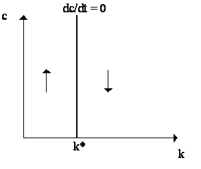
We can decipher the solution diagramatically in (c, k) space. Consider the dc/dt equation first (Figure 1). In steady-state, dc/dt = 0, implying that -(uc/ucc)·[¦k - r ] = 0. Now, making the reasonable assumption on the utility function that uc > 0 and that ucc < 0 for all positive c, then it must be that ¦k = r when dc/dt = 0. But this gives no clue as to what c thus c is indeterminate and the isokine dc/dt = 0 must be a straight vertical line, as shown in Figure 1. Where it intersects the horizontal axis, k*, can be deciphered if we assume ¦k is invertible, specifically:
we we see in Figure 1. If we assume ¦ (·) is Cobb-Douglas, so ¦ (k) = ka , then ¦k = aka-1 and so the dc/dt = 0 isokine intersects the horizontal axis at k* = (r /a )1/(a -1).
The disequilibrium dynamics are easily deciphered. From dc/dt = -(uc/ucc)·[¦ k - r ], recognize that:
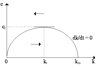
as uc > 0 and ucc, ¦ kk < 0. Thus, if k rises above k*, then c will automatically increase; conversely, if k is below k*, then c will fall. The directional arrows to the right and left of the dc/dt = 0 isokine in Figure 1 indicate these disequilibrium dynamics. Let us now turn to the second differential equation, dk/dt = ¦ (k) - c - nk. If dk/dt = 0, then c = ¦ (k) - nk. Thus, in (c, k) space as shown in Figure 2, the isokine dk/dt = 0 will be a concave function beginning at the origin (where c, k = 0) and intersecting the horizontal axis at km, where ¦ (km) = nkm (and thus c = 0). The slope of this isokine is ¦ k - n, thus the concave shape arises because of the diminishing marginal productivity of capital.
For the disequilibrium dynamics of the dk/dt = 0 isokine, notice that:
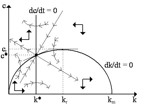
so anywhere above the dk/dt = 0 isokine, k falls, while anywhere underneath it, k rises. The horizontal arrows in Figure 2 indicate the disequilibrium dynamics. A point of interest is capital-labor ratio kr in Figure 2. This is where the isokine dk/dt = 0 yields its maximum consumption per capita, cr. At kr, notice that the slope of the dk/dt = 0 isokine is zero, thus ¦ k = n, the condition for Golden Rule growth we deciphered before. Thus, (kr, cr) are the Golden Rule capital-labor ratio and consumption per capita. We can combine the two isokines in Figure 3 to obtain the system as a whole. As we see, the steady-state equilibrium, where dc/dt = 0 and dk/dt = 0, will be at (k*, c*) in Figure 3, at the intersection of the isokines. Notice that this is below the Golden Rule equilibrium (kr, cr). We know that the isokine dc/dt = 0 lies to the left of kr because, recall, the isokine intersects the horizontal axis where ¦ k = r and we assumed before, for the integral to converge, that r > n, so at the steady-state equilibrium, ¦ k(k*) > n. Notice here that our solution will be Golden Rule growth if r = n. [Note: if we employed the Cass social welfare function with discount rate r rather than (r -n), we would then obtain Cass's "modified golden rule" ¦ k = r + n as our solution. In this case, we recover the Golden Rule as a solution if it happens that r = 0. Intriguingly, the Cass formulation (almost) reinforces Pigou's (1928) argument that time preference "contaminates" our system and makes savings "too low"! Purging our system of it will, as Pigou argued, lead to the "better" solution of Golden Rule growth. Incidentally, the Arrow-Kurz solution ¦ k = r is identical to that of the "static" model of Irving Fisher (1930: Ch.5).]
The dynamics of the depicted by using the directional arrows of our combined system to decipher the disequilibrium paths. This is a saddle-point dynamics: specifically, there is a single stable arm that goes to the steady-state (c*, k*) equilibrium; all other paths move away from this equilibrium. So what is the optimal path? This can be deciphered intuitively: namely, starting from any initial capital-labor ratio, k0, the "optimal" path would be to immediately set consumption c(0) so that we jump to the stable arm and, over time, approach (and reach) the equilibrium (c*, k*), and thereafter stay there forever. How do we know this is true? Intuitively, notice that if we sit on any other path, then we will go to one of two places: to the corner (0, km) on the horizontal axis or to the vertical axis (c, 0). But notice that in either case, consumption will eventually end. Going to the corner (0, km), consumption declines to zero -- and we consume zero forever after. Similarly, going to the vertical axis, we reach k = 0, and so, with no capital, we will gradually be brought down the axis to the origin so that consumption goes to zero. Thus, any path (except for the stable arms of the saddlepoint) will take us to zero consumption in finite time. Now, even if households discount the future heavily, it still has some weight in their utility. They will certainly not relish the prospect that after some finite amount of time, they will consume nothing forever after. Thus, only by "jumping" to one of the stable arms and going to the steady-state equilibrium (c*, k*) are they ensured that their consumption will be positive forever. Thus the "optimal" path will be that one. Mathematically, we know this is the case from the transversality condition. Specifically, for this problem, this is limt® ¥ l(t)e-rt = 0. But recall from the first order condition, that l = uc, so limt® ¥ uce-rt = 0. Now, for this to be true, then necessarily limt® ¥ uc < ¥ , i.e. the limit of marginal utility must be finite. But if consumption gets driven to zero (as all paths except the stable arm imply), then marginal utility will get driven to infinity. (as, by assumption, uc = ¥ when c = 0). Thus, the optimal path must, in the limit, not be at zero consumption. The only path which fulfills this transversality condition is the stable arm. We can confirm saddlepoint stability by examining the determinant of a linearization of our dynamic system. To simplify our notation, let us assume that utility has constant relative risk aversion (CRRA) form, i.e.
Notice that uc = c-g and ucc = -gc-g -1, so, by the Arrow-Pratt measure of relative risk-aversion:
thus the coeffient of relative risk aversion, g , is a constant. Now, we had a differential equation dc/dt = -(uc/ucc)·[¦ k - r ], so, assuming the CRRA functional form, this can now be rewritten
This makes linearization simpler. Namely, our system of differential equations can be rewritten as:
The determinant of the matrix of coefficients (call it J) is:
but as the coefficients are evaluated at equilibrium (c*, k*), then necessarily ¦k = r , so the determinant gets reduced to:
which is a sufficient condition for a saddlepoint dynamic system, exactly as we have drawn it in Figure 3. There are two more points of interest here. The first is that we have obtained a form of the Keynes-Ramsey rule. Specifically, consider our equation:
and let us rewrite it as:
Now, recall that ucc·(dc/dt) = duc/dt, so -(duc/dt)/uc = ¦k - r , so, setting r = 0 (consistent with Ramsey), then:
This, we claim, is a form of the Keynes-Ramsey rule. To understand this, recall that the Keynes-Ramsey rule stated that the marginal benefit of increasing savings is the net benefit of "faster" convergence to bliss, but the marginal cost of this would be the foregone consumption in the interim. There is no "bliss" in the Cass-Koopmans model, but there are future gains in utility. So, in discrete time, suppose that at time t, the social planner reduces consumption by the tiny amount dct, so that the loss of utility today is u¢(ct)·dct. This is the marginal cost of saving dct more. The marginal gain is the increase in utility tomorrow (t+1). The exact increase in consumption will be the amount dct transferred plus the extra productivity from that unit, i.e. dct + ¦ kdct So, the utility gain tomorrow will be dct·[1 + ¦ k]·u¢ (ct+1). As Keynes-Ramsey rule argues the marginal benefit of saving dct must be equal to its marginal cost, then
or, rearranging:
which states that the marginal product of capital (¦k) must equal the (proportional) decline in the marginal utility of consumption. Making the time difference short enough, we obtain:
which is what we had before. In effect, the Keynes-Ramsey rule is merely an extension of the Paretian "product mix efficiency" rule to an intertemporal scenario. Recall that it posited that the marginal rate of substitution between goods must be equal to the marginal rate of product transformation (MRS = MPT). The Keynes-Ramsey rule says the same thing, except that now we are comparing goods across periods,. so we must compare the marginal rate of substitution between periods (MRS = u¢(ct)/u¢(ct+1)) and the marginal rate of product transformation between periods, MPT = (1+¦k). Now, examine the discrete-time Keynes-Ramsey rule once more. Note that as ¦ k > 0, then it must be that u¢ (ct) - u¢ (ct+1) > 0. How is this justified? The simplest way is to claim that consumption is increasing over time (ct < ct+1), so that, automatically, the marginal utility of consumption declines, so u¢ (ct) > u¢ (ct+1), and we are done. This is legitimate, but we could also posit "time preference" in the utility function, i.e. that for the same c, ut(c) > ut+1(c). This implies that if ct = ct+1, then ut¢ (ct) < ut+1¢ (ct+1) automatically. Thus:
which is the Keynes-Ramsey rule. So, going back to our original equation (and assuming CRRA form for simplicity):
then we can reinterpret this as saying that consumption rises if the marginal product of capital exceeds the rate of time preference. This makes sense: the greater the marginal product of capital relative to time preference, the more worthwhile it is to decrease consumption now in order to increase consumption tomorrow (i.e. you "steepen" the consumption path so as to reach balanced growth quicker). A second point worth noting is that the equation ¦k = r + g (dc/dt)/c captures Eugen von Böhm-Bawerk's (1889) famous "three justifications" for the existence of interest or agio. The term g ·(dc/dt)/c captures "differences in want and provision for want" (a decrease in the marginal utility of consumption, due to growth); the time preference term r captures the systematic "underestimation of the future" and (perhaps a bit more arguably), the marginal productivity factor, ¦ k captures his "technical superiority of present goods". (cf. R. Frisch, 1964)
|
All rights reserved, Gonçalo L. Fonseca


